Automatic differentiation in Ruby
Contents
Introduction
Automatic differentiation is a clever trick that makes it easy to do differentiation on a computer. It’s a beautiful fusion of maths and computer programming, and I want to tell you about it so you can enjoy how satisfying it is.
“Differentiation” is a mathematical word for something we do to functions, so first we need to talk about what a function is.
What is a function?
A function really just means a relationship between two quantities — for example, the relationship between the current time and the distance travelled by a car.

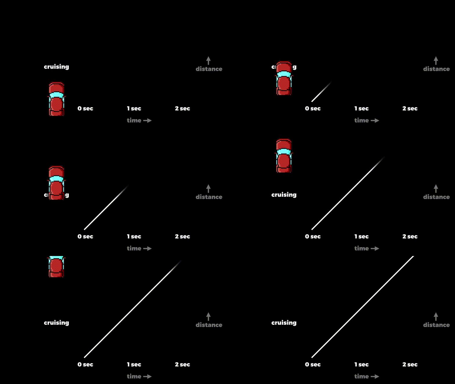
One relationship between time and distance might be “cruising along the road at a constant speed”, like the red car above. A different relationship is “pulling away from stationary”, like the green car — it starts slowly and speeds up. Each car has its own function that relates the distance it’s travelled to the current time.
If we plot time horizontally and distance vertically, the function of the red car’s distance over time looks like a straight line:
And the green car’s function looks like a curve:

If we periodically measure the red car’s distance we can get a sense of how it relates to the current time, and in this case we can see that the distance is actually equal to how many seconds it’s been travelling for:
| time | distance(time) |
|---|---|
| 0 seconds | 0 metres |
| 1 second | 1 metre |
| 2 seconds | 2 metres |
| 3 seconds | 3 metres |
| 4 seconds | 4 metres |
| ⋮ | ⋮ |
After three seconds it’s travelled three metres, for example.
If we measure the green car’s distance, it turns out it’s the time multiplied by itself:
| time | distance(time) |
|---|---|
| 0 seconds | 0 metres |
| 1 second | 1 metre |
| 2 seconds | 4 metres |
| 3 seconds | 9 metres |
| 4 seconds | 16 metres |
| ⋮ | ⋮ |
This time, after three seconds it’s travelled nine metres.
What is differentiation?
Differentiation is the process of finding out how fast a function’s result is changing, and to keep this article short, you’ll just have to believe me that this is a useful thing to be able to do on a computer.
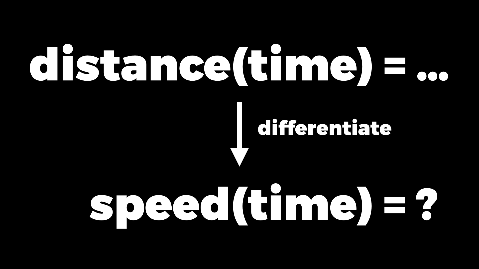
If we take a distance function and differentiate it, we get another function that tells us how fast the distance is changing, which in physics we call “speed”.
We know how far the green car has travelled at each point in time, but differentiation can tell us how fast it’s going at each point in time, which is otherwise not obvious:
| time | distance(time) | speed(time) |
|---|---|---|
| 0 seconds | 0 metres | ? |
| 1 second | 1 metre | ? |
| 2 seconds | 4 metres | ? |
| 3 seconds | 9 metres | ? |
| 4 seconds | 16 metres | ? |
| ⋮ | ⋮ | ⋮ |
We can see visually how fast a function is changing by graphing it and looking at the slope of the line:
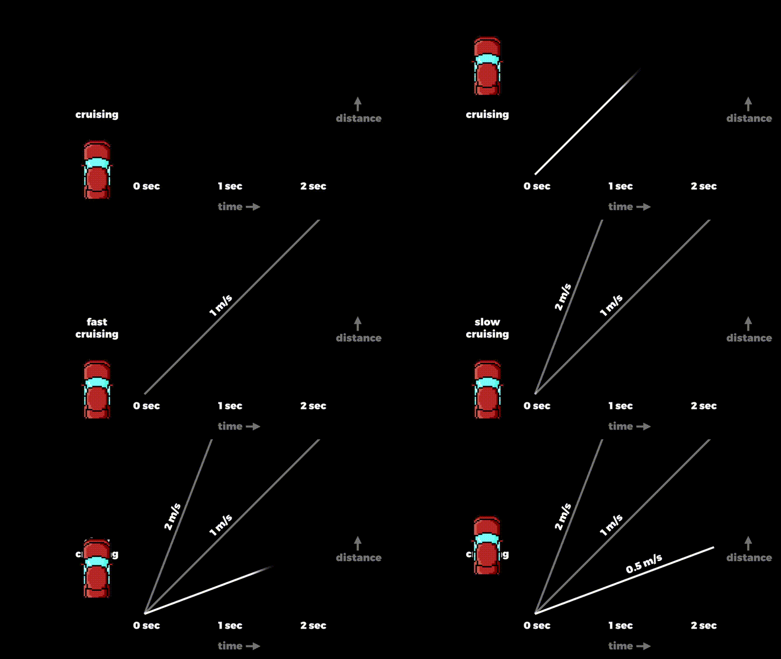
The red car’s distance function makes a straight line. Let’s say the slope is one metre per second: for every one second you go across, it goes one metre up. If the car travels twice as fast, the line is steeper; we can call that slope two metres per second. And if it travels half as fast, we get a less steep line, say half a metre per second. So steeper means faster, shallower means slower.
The speed of the green car changes over time.
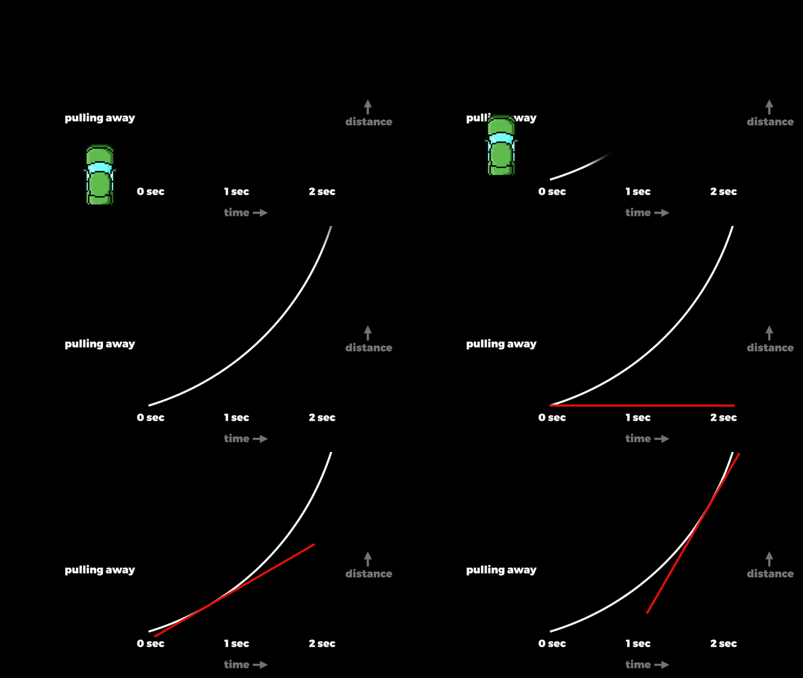
Initially its speed is zero, but then the curve gets steeper, and then even steeper as its speed increases.
Traditional strategies
So if we know these distance functions, how do we get a computer to calculate the speeds? There are two traditional ways of doing it.
Symbolic differentiation
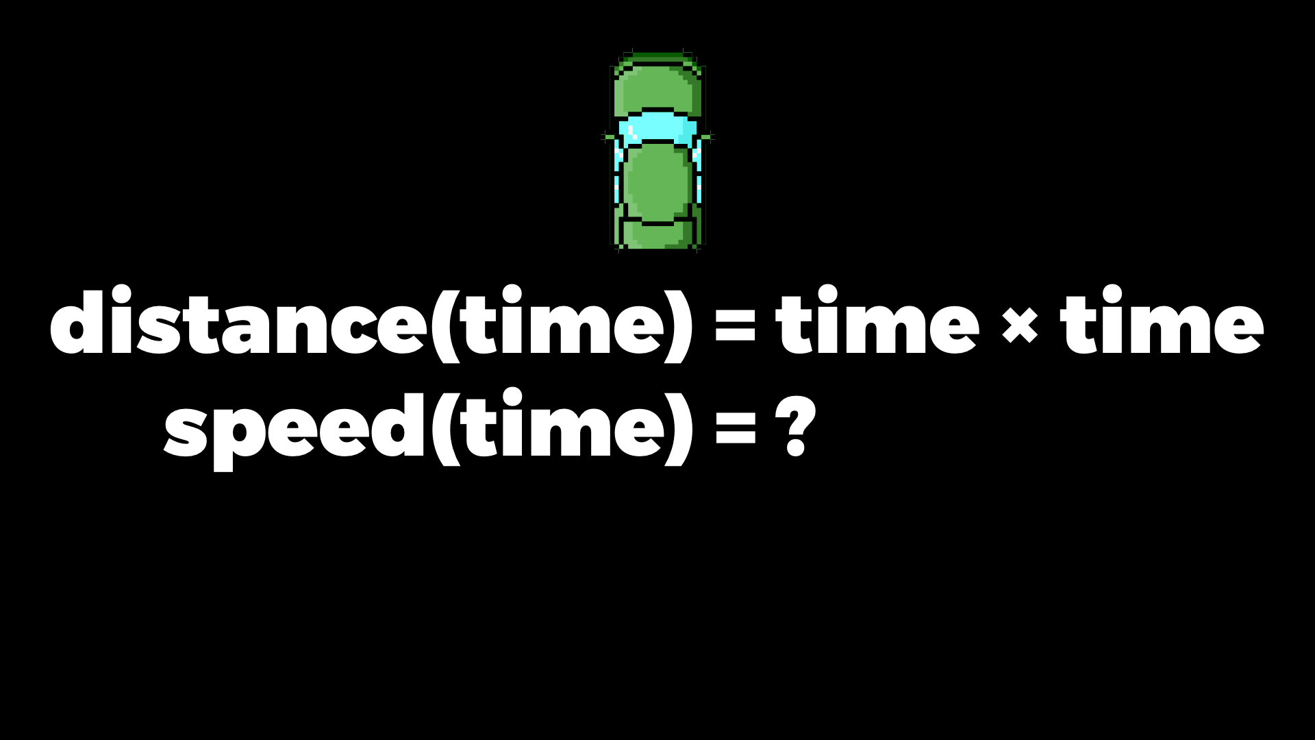
The first is called symbolic differentiation. The idea is to start with the expression of the function you want to differentiate — for example, “time × time” — and work out an expression for the differentiated function.
If you did any calculus at school, you’ll know that mathematicians have a load of rules for how to do these manipulations. There’s a whole Wikipedia page full of them: the constant factor rule, the sum rule, the subtraction rule, the product rule, the chain rule, the inverse function rule, the elementary power rule, and so on.
To do symbolic differentiation, we represent the expression as a data structure inside the computer — as a tree of symbols — and get the computer to manipulate that structure according to all those differentiation rules and the rules of basic algebra.
Firstly, we teach the computer that “time × time” can be written as “time²” — time to the power of two. And then one of the differentiation rules, the elementary power rule, says: something to the power of n differentiates to n multiplied by that something to the power of n - 1:
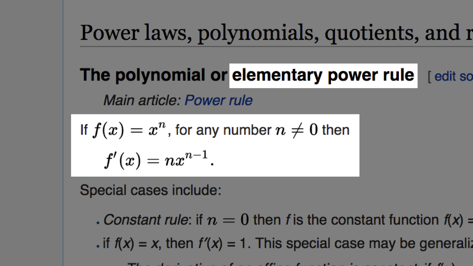
So time to the power of two differentiates to two multiplied by time to the power of one, which is just 2 × time.
Now we know that speed is 2 × time, we can compute the speeds:
| time | distance(time) | speed(time) |
|---|---|---|
| 0 seconds | 0 metres | 0 m/s |
| 1 second | 1 metre | 2 m/s |
| 2 seconds | 4 metres | 4 m/s |
| 3 seconds | 9 metres | 6 m/s |
| 4 seconds | 16 metres | 8 m/s |
| ⋮ | ⋮ | ⋮ |
So the big picture is: from the expression for distance, the computer uses some rules to work out the expression for speed, and then evaluates it for different inputs. That gives accurate answers but it’s difficult to do. Also, in general, the size of the differentiated expression can be much larger than the size of the original expression, so it takes longer to evaluate.
Numerical differentiation
The other traditional strategy is called numerical differentiation. Instead of representing the function’s expression as a data structure, we implement it directly as a program.
Here’s the green car’s distance function in Ruby:
def distance(time:)
  time * time
end
The idea of numerical differentiation is that we can guess the rate of change at a particular value by picking a nearby value and looking at the slope of the line that connects them:
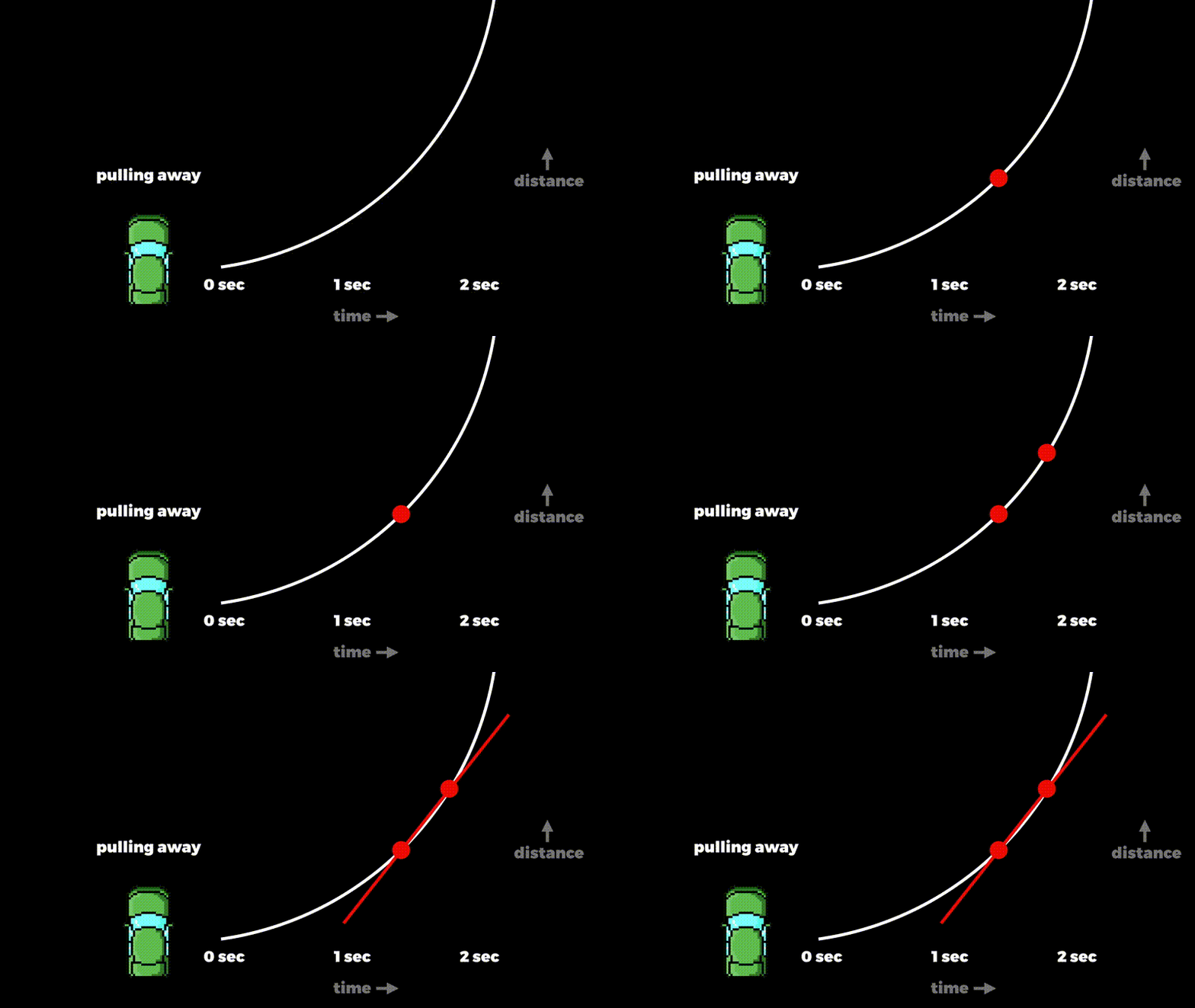
The slope of that line doesn’t quite match the curve, so it’s only an approximation. On the other hand, if we choose an even closer value the approximation gets more accurate. It’ll never be perfect, but if we pick a small enough distance between the two values, the line between them matches the slope of the curve quite closely:
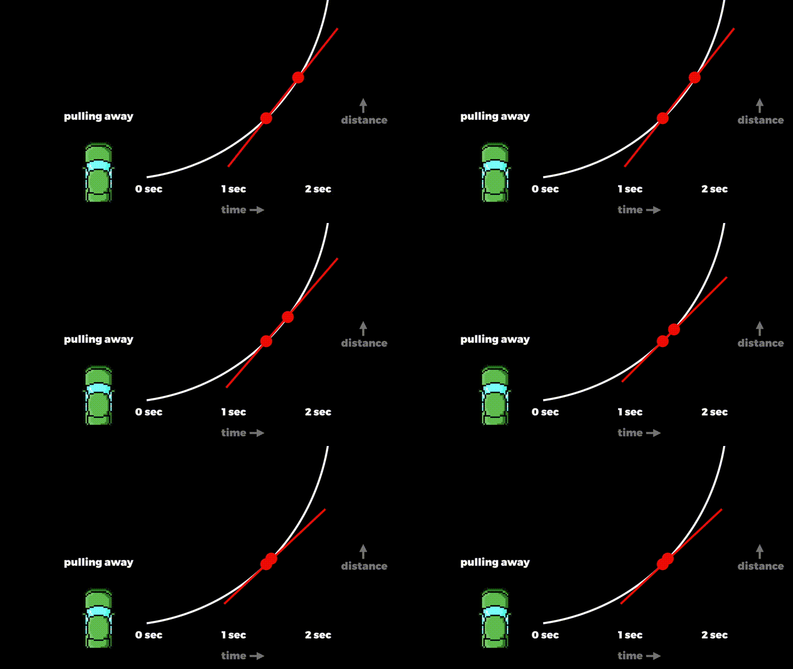
Here’s how we implement it:
def speed(time:)
  time_elapsed = 0.01

  distance_before = distance(time: time)
  distance_after  = distance(time: time + time_elapsed)

  distance_travelled = distance_after - distance_before

  distance_travelled / time_elapsed
end
To get the rough speed at a particular time, we pick a really short amount of time — say, 0.01 seconds — then calculate how much further the car travels in that time, and divide that distance by the amount of time elapsed. We don’t need to reimplement this for every function we want to differentiate; we can make a higher order function to do it, or do it with metaprogramming or whatever.
Here are the results of our speed method:
>>speed(time: 0)=> 0.01 >>speed(time: 1)=> 2.0100000000000007 >>speed(time: 2)=> 4.009999999999891 >>speed(time: 3)=> 6.009999999999849 >>speed(time: 4)=> 8.009999999999806
They’re extremely close to the exact answers we got from doing it symbolically.
With this technique we don’t have a simple expression that tells us the speed directly, but we do have an algorithm that lets us approximate it:
| time | distance(time) | speed(time) |
|---|---|---|
| 0 seconds | 0 metres | 0.01 m/s |
| 1 second | 1 metre | 2.01 m/s |
| 2 seconds | 4 metres | 4.01 m/s |
| 3 seconds | 9 metres | 6.01 m/s |
| 4 seconds | 16 metres | 8.01 m/s |
| ⋮ | ⋮ | ⋮ |
This is easier and faster than the symbolic method, but it’s only approximate, and dividing by tiny quantities makes it susceptible to rounding errors.
Automatic differentiation
We’ve seen the traditional strategies: symbolic and numerical differentiation. Automatic differentiation is a less well-known technique. It’s almost as accurate as symbolic differentiation but as fast and easy as numerical.
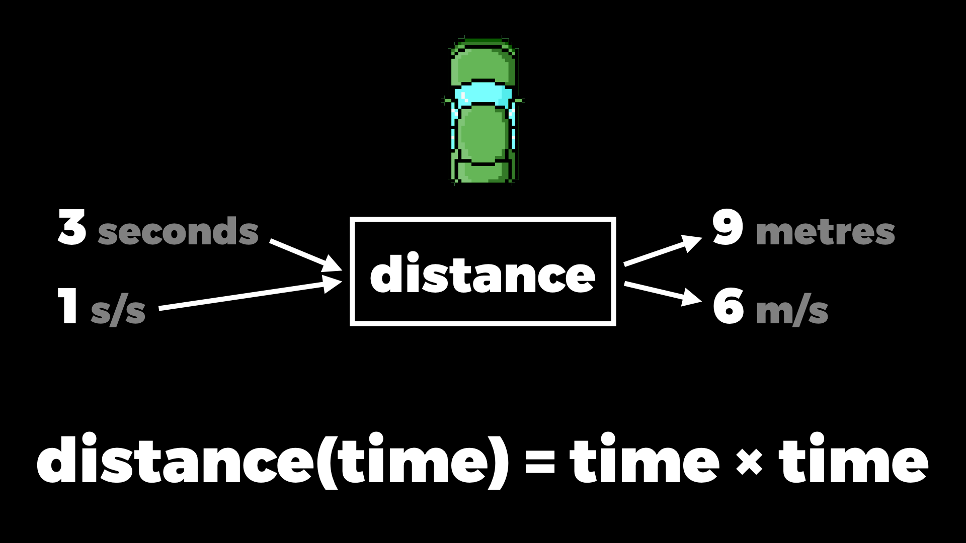
The big idea is to calculate a function’s rate of change and its value all at once. Rather than putting a time into our distance function and getting a distance out, we should put in a time and a rate of change — for example, we specify that time is changing at one second per second — and get out a distance and a rate of change — for example, we get the result that the distance is changing at six metres per second.
Dual numbers
One way of doing this is to invent a new kind of number that can represent a value and its rate of change together, and then make our implementations of functions work with these new numbers. So we need to design and then implement a sort of two-dimensional number that can store both a value and its rate of change and operate on them simultaneously.
One kind of two-dimensional number you might already know about is the complex numbers, which were invented to solve a similar problem. They have two components, a real part and an imaginary part, but they can be added and multiplied and otherwise used like normal numbers. The imaginary part of a complex number is a multiple of the invented number i — it’s just a symbol, it doesn’t represent a real quantity.
Our two-dimensional numbers will use a similar idea, but they’re not complex numbers, they’re called dual numbers. They have a real part and a dual part, and instead of i we use the invented number ε (the Greek letter epsilon). It’s just a symbol again, but you can think of ε as representing a very very tiny number, almost zero but not zero — it’s called an infinitesimal.
We’ll use this dual part to represent the rate at which a number is changing. ε is so tiny that it doesn’t contribute to the real value of the number at all, but we can say a number with 10ε is changing twice as fast as a number with 5ε.
So let’s just make a boring class for dual numbers, with accessors for the real and dual parts, and a string representation:
class DualNumber
  attr_accessor :real, :dual

  def initialize(real:, dual:)
    self.real = real
    self.dual = dual
  end

  def to_s
    [real, (dual < 0 ? '-' : '+'), dual.abs, 'ε'].join
  end

  def inspect
    "(#{to_s})"
  end
end
And add a convenience method to Kernel for converting normal numbers into dual numbers, like the Complex and Rational classes have:
module Kernel
  def DualNumber(real, dual = 0)
    case real
    when DualNumber
      real
    else
      DualNumber.new(real: real, dual: dual)
    end
  end
end
If we don’t specify a rate of change then it defaults to zero. That gives us a dual number that represents a constant — a value that’s not changing at all.
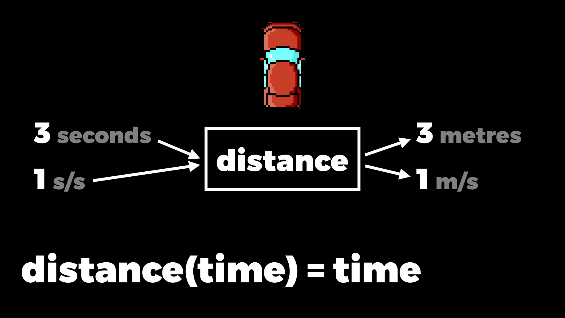
So for the red car, where the distance is just equal to the time, we already have something that works. We make a value three with rate of change one, and when we call the distance function with it, we get out three with rate of change one — that means three metres, one metre per second:
def distance(time:)
  time
end>>time_now = DualNumber(3, 1)=> (3+1ε) >>distance_now = distance(time: time_now)=> (3+1ε) >>distance_now.real=> 3 >>distance_now.dual=> 1
And that’s the right answer for this very simple function where distance is the same as time.
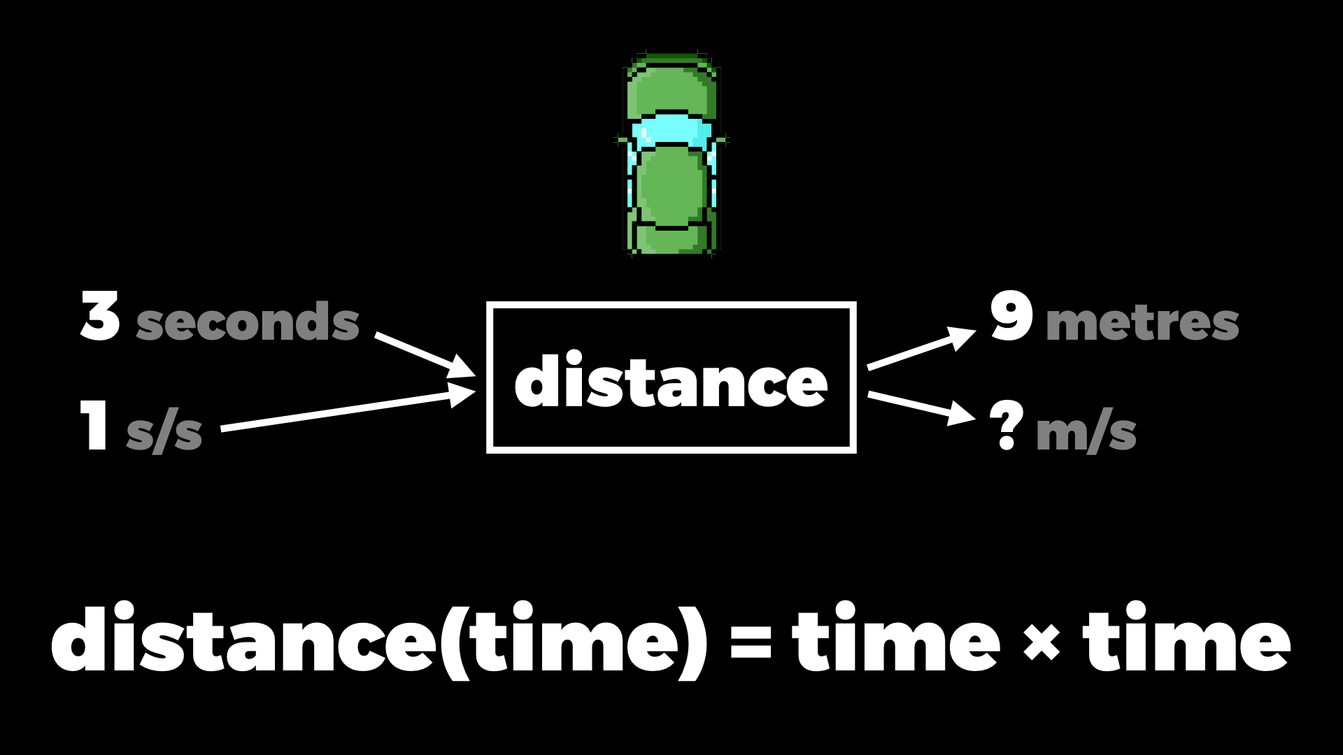
But what about when the function does some operations on the input value?
Adding and multiplying
If you’ve worked with complex numbers you might know that we can define how to add and multiply them, and so on, just by doing normal algebra with their parts. But to do that we need to know how i behaves, and by design the rule is that i × i = -1. That choice makes complex numbers behave in a certain way; they’re good for representing rotations and oscillations and things like that in physics and electronics.
We can add together two complex numbers by just adding all their parts separately and grouping the multiples of i together:
| (a + bi) + (c + di) | = | a + c + bi + di |
| = | (a + c) + (b + d)i |
And when we multiply two complex numbers we multiply out the brackets and group the multiples of i:
| (a + bi) × (c + di) | = | (a × c) + (a × di) + (bi × c) + (bi × di) |
| = | ac + (ad + bc)i + bdi² | |
| = | ac + (ad + bc)i - bd | |
| = | (ac - bd) + (ad + bc)i |
We end up multiplying by i² at the end of the second line, and that just turns into multiplying by -1 because that’s what i² is, so that becomes a subtraction, and then we group the multiples again.
We can do exactly the same thing for dual numbers too, but this time we need to know how ε behaves. The rule for ε is that it’s so small that when you multiply it by itself you get zero. And then all the algebra follows in the same way.
Adding dual numbers is literally the same. We add all the parts and group the multiples of ε:
| (a + bε) + (c + dε) | = | a + c + bε + dε |
| = | (a + c) + (b + d)ε |
Multiplying is almost the same. We multiply out the brackets and group the multiples, but now we’re multiplying by ε² at the end, and ε² is zero, so that last part just goes away:
| (a + bε) × (c + dε) | = | (a × c) + (a × dε) + (bε × c) + (bε × dε) |
| = | ac + (ad + bc)ε + bdε² | |
| = | ac + (ad + bc)ε + bd × 0 | |
| = | ac + (ad + bc)ε |
We can use those results to implement + and * on our DualNumber class. This is where the mathematics meets the programming:
class DualNumber
  def +(other)
    DualNumber.new \
      real: real + other.real,
      dual: dual + other.dual
  end

  def *(other)
    DualNumber.new \
      real: real * other.real,
      dual: real * other.dual + dual * other.real
  end
end
Now if we have two dual numbers, we can add them and multiply them:
>>x = DualNumber(1, 2)=> (1+2ε) >>y = DualNumber(3, 4)=> (3+4ε) >>x + y=> (4+6ε) >>x * y=> (3+10ε)
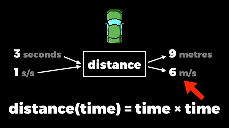
So for the green car, where the distance is time multiplied by time, we can take that three seconds changing at one second per second, ask for the distance, and get the result: nine metres changing at six metres per second.
def distance(time:)
  time * time
end>>time_now = DualNumber(3, 1)=> (3+1ε) >>distance_now = distance(time: time_now)=> (9+6ε) >>distance_now.real=> 9 >>distance_now.dual=> 6
And that’s the answer we wanted. It just works, because we built the idea of the rate of change into our numbers, and defined operations that preserved and respected the rate of change.
Here’s what we see if we feed different time values into the green car’s distance function and visualise the dual numbers it generates:
The real values are plotted in black, and the slope of the red line is the dual part — the rate of change for the value where the dot is. So you can see that matches the slope of the curve nicely.
Compatibility
We have to do a bit of work to make dual numbers compatible with Ruby’s built-in numbers. Right now if we try to add or multiply by a Fixnum we get a NoMethodError, because our add and multiply operations are trying to get the real and dual parts of a Fixnum:
>>x = DualNumber(1, 2)=> (1+2ε) >>(x + 3) * 4NoMethodError: undefined method `dual' for 3:Fixnum
We can fix that by just converting the argument to a dual number inside the add and multiply methods. This is where that DualNumber conversion method comes in handy:
class DualNumber
  def +(other)
    other = DualNumber(other)

    DualNumber.new \
      real: real + other.real,
      dual: dual + other.dual
  end

  def *(other)
    other = DualNumber(other)

    DualNumber.new \
      real: real * other.real,
      dual: real * other.dual + dual * other.real
  end
end
And now we can add and multiply by normal numbers. They get automatically converted into dual number constants:
>>x = DualNumber(1, 2)=> (1+2ε) >>(x + 3) * 4=> (16+8ε)
Of course we have the opposite problem, too, if we have a Fixnum on the left and try to add or multiply by a dual number on the right. This time instead of a NoMethodError we get a TypeError, because Fixnum’s add and multiply operations don’t know what to do with a dual number:
>>x = DualNumber(1, 2)=> (1+2ε) >>3 + (4 * x)TypeError: DualNumber can't be coerced into Fixnum
Fortunately Ruby has a built-in way of coping with this. If we call a numeric operation of a built-in number with an argument whose type it doesn’t recognise, the number will send a coerce message to that unrecognised argument, and expect to get back a pair of objects. Then it will retry the original operation with those objects, and whatever result it gets back, it will return that.
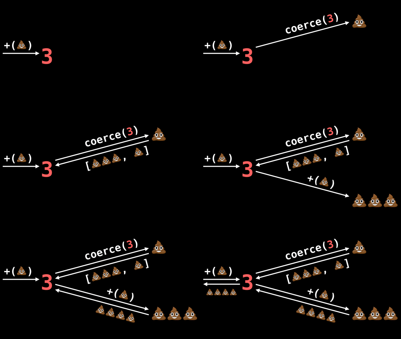
This coercion protocol means built-in numbers can interoperate with user-defined ones.
So if we implement this coerce method on the DualNumber class, we can make built-in numbers automatically upgrade themselves to a dual number whenever we try to add or multiply by a dual number:
class DualNumber
  def coerce(other)
    [DualNumber(other), self]
  end
end
And now addition and multiplication work both ways around:
>>x = DualNumber(1, 2)=> (1+2ε) >>3 + (4 * x)=> (7+8ε)
Other functions
Of course, you can do more with numbers than just add and multiply them. With a bit more algebra it’s possible to work out definitions for all sorts of other operations on dual numbers too. For example, these are the formulas for taking the sine, cosine, natural exponential, natural logarithm and square root of a dual number:
| sin(a + bε) | = | sin(a) + (b × cos(a))ε |
| cos(a + bε) | = | cos(a) - (b × sin(a))ε |
| exp(a + bε) | = | exp(a) + (b × exp(a))ε |
| log(a + bε) | = | log(a) + (b ÷ a)ε |
| sqrt(a + bε) | = | sqrt(a) + (b ÷ (2 × sqrt(a))ε |
Those formulas are easy to monkey patch into the Math module:
Math.singleton_class.prepend Module.new {
  def sin(x)
    case x
    when DualNumber
      DualNumber.new \
        real: sin(x.real),
        dual: x.dual * cos(x.real)
    else
      super
    end
  end

  def cos(x)
    case x
    when DualNumber
      DualNumber.new \
        real: cos(x.real),
        dual: -x.dual * sin(x.real)
    else
      super
    end
  end
}
Here we’re overriding sin and cos in the Math module to use the appropriate formulas if they’re called with a dual number, otherwise they call super to use the original implementation.
Now we can take the sine and cosine of dual numbers, and combine them into larger expressions:
>>x = DualNumber(Math::PI / 3, 1)=> (1.0471975511965976+1ε) >>Math.sin(x)=> (0.8660254037844386+0.5000000000000001ε) >>Math.sin(x) + Math.cos(x)=> (1.3660254037844388-0.3660254037844385ε) >>Math.sin(x) * Math.cos(x / 2)=> (0.75+0.21650635094610984ε)
If we define the distance function to be the sine of the time…
def distance(time:)
  Math.sin(time)
end
…then here’s the graph of the real and dual values that the Ruby code produces. Hopefully you’re convinced that the slope of the line is correct.
And we can compose as many operations as we want. Here’s a distance function that does sine and cosine and multiplies and adds and divides…
def distance(time:)
  Math.sin(time) * 0.8 + Math.cos(time * 5) / 5
end
…and here are the values and rates of change produced by that code:
Here’s a final example:
def distance(time:)
  time * Math.sin(time * time) + 1
end
time × sin(time²) + 1 looks like this:
Conclusion
So that’s it. A clever little trick that works by inventing a new kind of number, defining operations on it that preserve its meaning, and passing it into existing functions to see what they do to it. The Ruby dual number implementation I built for this article is available on GitHub, or you can install it as a gem if you want to play around with it.