Compilers for Free

Introduction
Execution
Interpretation
Compilation
Partial evaluation
Applications
The Futamura projections
Conclusion

Introduction

I’m fascinated by programming, and by metaprogramming in particular. When Ruby programmers talk about metaprogramming they usually mean programs that write programs, because Ruby has various features — like BasicObject#instance_eval, Module#define_method and BasicObject#method_missing — which make it possible to write programs that grow new functionality at run time.

But there’s another aspect of metaprogramming that I find even more interesting: programs that manipulate representations of programs. These are programs which ingest data that itself represents a program, and then do something with that representation, like analyse it, evaluate it, translate it, or transform it.

This is the world of interpreters, compilers and static analysers, and I think it’s fascinating. It’s the purest and most self-referential kind of software that we can write.

By showing you around this world I’d like to make you look at programs differently. I don’t have a complicated technical point to make; I just want to tell you a cool story, show you that programs which manipulate other programs are interesting, and hopefully inspire you to find out some more about them.

Execution

We’ll begin by considering something easy and familiar: executing programs.

Say we have a program that we want to run, as well as a machine to run it on. To execute the program, the first step is to put the program into the machine. Then we have some inputs for that program — command-line arguments, or configuration files, or standard input, or whatever — so we feed all of those inputs into the machine too.

In principle, the program executes on the machine, reads the inputs, and produces some output:

An animation showing a program reading input to produce output

In practice, though, this simple picture is only possible if the program is written in a language that the machine can execute directly. For a bare-metal physical machine that means the program has to be written in low-level machine code. (If the program’s written in a higher-level language then we may be able to run it on a virtual machine that understands that language natively, e.g. Java bytecode on the JVM.)

But if our program’s written in a language that’s unfamiliar to the machine, we can’t execute it directly; we need an interpreter or compiler.

Interpretation

An interpreter works roughly like this:

it reads in the source code of the program we want to execute; then
it builds an abstract syntax tree (AST) by parsing that source code; and finally
it evaluates the program by walking over the abstract syntax tree and performing the instructions that it finds.

Let’s investigate each of those steps by building an interpreter for a toy language called Simple (“simple imperative language”). It’s very straightforward and looks a little bit like Ruby, but it’s not exactly the same. Here are some example Simple programs:

a = 19 + 23

x = 2; y = x * 3

if (a < 10) { a = 0; b = 0 } else { b = 10 }

x = 1; while (x < 5) { x = x * 3 }

Unlike Ruby, Simple makes a distinction between expressions and statements. An expression evaluates to a value; for example, the expression 19 + 23 evaluates to 42, and the expression x * 3 evaluates to three times whatever the current value of the variable x is. On the other hand, evaluating a statement doesn’t produce a value, but it has the side effect of updating the current values of variables; evaluating the assignment statement a = 19 + 23 updates the variable a to have the value 42.

As well as assignment, Simple has a few other kinds of statement: sequencing (evaluating one statement before evaluating another, i.e. the semicolon), conditionals (if (…) { … } else { … }), and loops (while (…) { … }). These kinds of statement don’t directly affect the values of variables, but they can all contain nested assignment statements which do.

There’s a Ruby library called Treetop which makes it easy to build parsers, so we’re going to quickly use Treetop to build a parser for Simple. (We won’t go into any of the gory details here — have a look at the Treetop documentation if you’d like to know more.)

To use Treetop we have to write a file called a grammar, which looks like this:

grammar Simple
  rule statement
    sequence
  end

  rule sequence
    first:sequenced_statement '; ' second:sequence
    /
    sequenced_statement
  end

  rule sequenced_statement
    while / assign / if
  end

  rule while
    'while (' condition:expression ') { ' body:statement ' }'
  end

  rule assign
    name:[a-z]+ ' = ' expression
  end

  rule if
    'if (' condition:expression ') { ' consequence:statement
      ' } else { ' alternative:statement ' }'
  end

  rule expression
    less_than
  end

  rule less_than
    left:add ' < ' right:less_than
    /
    add
  end

  rule add
    left:multiply ' + ' right:add
    /
    multiply
  end

  rule multiply
    left:term ' * ' right:multiply
    /
    term
  end

  rule term
    number / boolean / variable
  end

  rule number
    [0-9]+
  end

  rule boolean
    ('true' / 'false') ![a-z]
  end

  rule variable
    [a-z]+
  end
end

This grammar contains rules which explain what each kind of Simple statement and expression looks like. The sequence rule means “a sequence is two statements separated by a semicolon”, the while rule means “a loop begins with ‘while (’, followed by a condition, followed by the loop’s body surrounded by curly braces”, the assignment rule means “an assignment looks like a variable name followed by an equals sign and an expression”, and so on. The number, boolean and variable rules explain that numbers are sequences of digits, booleans are written as “true” and “false”, and variable names are sequences of letters.

Once we’ve written a grammar, we can use Treetop to load it and generate a parser. The parser gets generated as a Ruby class, so we can instantiate that class and ask it to parse a string. Assuming that the above grammar has been saved into a file called simple.treetop, here’s how we do that in IRB:

>> Treetop.load('simple.treetop')
=> SimpleParser

>> SimpleParser.new.parse('x = 2; y = x * 3')
=> SyntaxNode+Sequence1+Sequence0 offset=0, "x = 2; y = x * 3" (first,second):
     SyntaxNode+Assign1+Assign0 offset=0, "x = 2" (name,expression):
       SyntaxNode offset=0, "x":
         SyntaxNode offset=0, "x"
       SyntaxNode offset=1, " = "
       SyntaxNode+Number0 offset=4, "2":
         SyntaxNode offset=4, "2"
     SyntaxNode offset=5, "; "
     SyntaxNode+Assign1+Assign0 offset=7, "y = x * 3" (name,expression):
       SyntaxNode offset=7, "y":
         SyntaxNode offset=7, "y"
       SyntaxNode offset=8, " = "
       SyntaxNode+Multiply1+Multiply0 offset=11, "x * 3" (left,right):
         SyntaxNode+Variable0 offset=11, "x":
           SyntaxNode offset=11, "x"
         SyntaxNode offset=12, " * "
         SyntaxNode+Number0 offset=15, "3":
           SyntaxNode offset=15, "3"

The parser produces a data structure called a concrete syntax tree, or a parse tree, which contains a lot of information about how the parsed string breaks down into all its component parts.

There’s a lot of fiddly detail in the concrete syntax tree that we’re not very interested in. In fact we don’t want a concrete syntax tree at all, we want an abstract syntax tree, which is a simpler and more useful representation of the structure of the program.

To make an abstract syntax tree, we first need to declare some classes that we’re going to use to build the tree’s nodes. That’s easy to do with Struct:

Number    = Struct.new :value
Boolean   = Struct.new :value
Variable  = Struct.new :name

Add       = Struct.new :left, :right
Multiply  = Struct.new :left, :right
LessThan  = Struct.new :left, :right

Assign    = Struct.new :name, :expression
If        = Struct.new :condition, :consequence, :alternative
Sequence  = Struct.new :first, :second
While     = Struct.new :condition, :body

Here we’re defining a new class for each different kind of expression and statement: simple expressions like Number and Boolean just have a value, binary expressions like Add and Multiply have a left and right subexpression, Assign statements have got the name of a variable and the expression to assign to it, and so on.

Treetop allows us to add functionality to the nodes of a concrete syntax tree by putting Ruby method definitions inside a grammar file’s rules. We can use this feature to give each kind of concrete syntax tree node a method that converts it into the corresponding kind of AST node; let’s call that method #to_ast.

Here’s how we define #to_ast for numbers, booleans and variables within the Simple grammar:

rule number
  [0-9]+ {
    def to_ast
      Number.new(text_value.to_i)
    end
  }
end

rule boolean
  ('true' / 'false') ![a-z] {
    def to_ast
      Boolean.new(text_value == 'true')
    end
  }
end

rule variable
  [a-z]+ {
    def to_ast
      Variable.new(text_value.to_sym)
    end
  }
end

When Treetop uses the number rule to build a node for the concrete syntax tree, that node will now come with an implementation of #to_ast which converts its textual content into an integer (using String#to_i) and then returns that integer wrapped in an instance of the Number class. The #to_ast implementations in the boolean and variable rules contain similar code to build an instance of the appropriate AST class containing the appropriate value.

Here are the #to_ast implementations for the three kinds of binary expression:

rule less_than
  left:add ' < ' right:less_than {
    def to_ast
      LessThan.new(left.to_ast, right.to_ast)
    end
  }
  /
  add
end

rule add
  left:multiply ' + ' right:add {
    def to_ast
      Add.new(left.to_ast, right.to_ast)
    end
  }
  /
  multiply
end

rule multiply
  left:term ' * ' right:multiply {
    def to_ast
      Multiply.new(left.to_ast, right.to_ast)
    end
  }
  /
  term
end

In all three cases, #to_ast recursively converts the concrete syntax trees representing the left and right subexpressions into ASTs by calling #to_ast on them, and then combines them into one overall AST node of the appropriate class.

Statements work similarly:

rule sequence
  first:sequenced_statement '; ' second:sequence {
    def to_ast
      Sequence.new(first.to_ast, second.to_ast)
    end
  }
  /
  sequenced_statement
end

rule while
  'while (' condition:expression ') { ' body:statement ' }' {
    def to_ast
      While.new(condition.to_ast, body.to_ast)
    end
  }
end

rule assign
  name:[a-z]+ ' = ' expression {
    def to_ast
      Assign.new(name.text_value.to_sym, expression.to_ast)
    end
  }
end

rule if
  'if (' condition:expression ') { ' consequence:statement
    ' } else { ' alternative:statement ' }' {
    def to_ast
      If.new(condition.to_ast, consequence.to_ast, alternative.to_ast)
    end
  }
end

Again, #to_ast simply converts each subexpression or substatement into an AST and glues the results together with the right kind of AST class.

Once all the definitions of #to_ast are in place, we can use Treetop to build a concrete syntax tree and then call #to_ast on the root node to recursively convert the whole thing into an AST:

>> SimpleParser.new.parse('x = 2; y = x * 3').to_ast
=> #<struct Sequence
     first=#<struct Assign
       name=:x,
       expression=#<struct Number value=2>
     >,
     second=#<struct Assign
       name=:y,
       expression=#<struct Multiply
         left=#<struct Variable name=:x>,
         right=#<struct Number value=3>
       >
     >
   >

Whereas Treetop’s detailed concrete syntax tree is designed for Treetop’s purposes, the AST is a simpler data structure built out of instances of classes that we designed ourselves. The AST for x = 2; y = x * 3 has this structure:

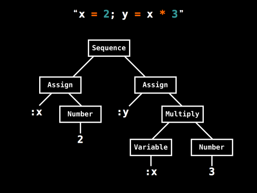
A diagram of an abstract syntax tree, showing the structure of the statement x = 2; y = x * 3

This tells us that the statement x = 2; y = x * 3 is a Sequence of two Assignments: the first Assignment is assigning the Number 2 to x, and the second Assignment is assigning the result of Multiplying the Variable x and the Number 3 to y.

Now that we’ve got this AST, we can evaluate it by recursively walking over it. On each AST node class we’ll define a method called #evaluate which performs the operations represented by that node and any of its subtrees; once that’s done, we can call #evaluate on the root node of the AST to evaluate the whole program.

Here’s what #evaluate looks like for Number, Boolean and Variable nodes:

class Number
  def evaluate(environment)
    value
  end
end

class Boolean
  def evaluate(environment)
    value
  end
end

class Variable
  def evaluate(environment)
    environment[name]
  end
end

The environment argument is a hash which contains the current value of each variable. An environment of { x: 7, y: 11 }, for example, means that there are two variables, x and y, with the values 7 and 11 respectively. We’ll assume that every Simple program is evaluated within some (possibly empty) initial environment; later we’ll see how statements can change the current environment.

When we’re evaluating a Number or Boolean we don’t care what’s in the environment, because we always just return the value that was stored inside that node when it was built. If we’re evaluating a Variable, though, we have to look in the environment and retrieve the current value of the variable with that name.

So if we make a new Number AST node and evaluate it in an empty environment, we get the original Ruby number back:

>> Number.new(3).evaluate({})
=> 3

The same goes for Booleans:

>> Boolean.new(false).evaluate({})
=> false

If we evaluate a Variable called y in an environment that gives y the value 11, the result will be 11, whereas if we evaluate it in an environment that gives y a different value we’ll get that value instead:

>> Variable.new(:y).evaluate({ x: 7, y: 11 })
=> 11

>> Variable.new(:y).evaluate({ x: 7, y: true })
=> true

Here are the definitions of #evaluate for binary expressions:

class Add
  def evaluate(environment)
    left.evaluate(environment) + right.evaluate(environment)
  end
end

class Multiply
  def evaluate(environment)
    left.evaluate(environment) * right.evaluate(environment)
  end
end

class LessThan
  def evaluate(environment)
    left.evaluate(environment) < right.evaluate(environment)
  end
end

These implementations recursively evaluate their left and right subexpressions and then perform the appropriate operation on the results. If it’s an Add node, the results are added; if it’s a Multiply they’re multiplied together; if it’s a LessThan, the results are compared using Ruby’s < operator.

So, when we evaluate the Multiply expression x * y in an environment that gives x the value 2 and y the value 3, we get the result 6:

>> Multiply.new(Variable.new(:x), Variable.new(:y)).
     evaluate({ x: 2, y: 3 })
=> 6

If we evaluate the LessThan expression x < y in the same environment, we get the result true:

>> LessThan.new(Variable.new(:x), Variable.new(:y)).
     evaluate({ x: 2, y: 3 })
=> true

For statements, #evaluate works slightly differently. Because evaluating a Simple statement updates the environment rather than returning a value, we define #evaluate to return a new environment hash that reflects any changes that the statement has made to the current values of variables.

The only kind of statement which directly affects variables is Assign:

class Assign
  def evaluate(environment)
    environment.merge({ name => expression.evaluate(environment) })
  end
end

To evaluate an Assign statement we first evaluate the right-hand side of the assignment to get a value, and then use Hash#merge to create a modified environment which associates that value with the appropriate variable name.

If we evaluate x = 2 in an empty environment, we get back a new environment which says the value of x is 2:

>> Assign.new(:x, Number.new(2)).evaluate({})
=> {:x=>2}

Similarly, if we evaluate y = x * 3 in an environment which says x is 2, then the subexpression x * 3 will evaluate to 6, resulting in an environment which says that x and y have the values 2 and 6 respectively:

>> Assign.new(:y, Multiply.new(Variable.new(:x), Number.new(3))).
     evaluate({ x: 2 })
=> {:x=>2, :y=>6}

We can evaluate a Sequence of two statements by evaluating the first statement to get an intermediate environment, then evaluating the second statement in that intermediate environment to get a final environment:

class Sequence
  def evaluate(environment)
    second.evaluate(first.evaluate(environment))
  end
end

In a Sequence of two assignments to the same variable, for example, the second assignment will win:

>> Sequence.new(
     Assign.new(:x, Number.new(1)),
     Assign.new(:x, Number.new(2))
   ).evaluate({})
=> {:x=>2}

Finally, we need definitions of #evaluate for If and While statements:

class If
  def evaluate(environment)
    if condition.evaluate(environment)
      consequence.evaluate(environment)
    else
      alternative.evaluate(environment)
    end
  end
end

class While
  def evaluate(environment)
    if condition.evaluate(environment)
      evaluate(body.evaluate(environment))
    else
      environment
    end
  end
end

If evaluates one of its two substatements depending on the value of its condition, and While uses recursion to repeatedly evaluate the loop body as long as its condition evaluates to true. (See “The Meaning of Programs” for a fuller explanation of how this works.)

Now that we’ve implemented #evaluate for each kind of expression and statement, we can parse any Simple program and evaluate the resulting AST. Let’s see what happens when we evaluate x = 2; y = x * 3 in an empty environment:

>> SimpleParser.new.parse('x = 2; y = x * 3').
     to_ast.evaluate({})
=> {:x=>2, :y=>6}

As expected, the final result is that x and y have the values 2 and 6.

Let’s try a more sophisticated program:

>> SimpleParser.new.parse('x = 1; while (x < 5) { x = x * 3 }').
     to_ast.evaluate({})
=> {:x=>9}

This program initialises x with 1, then repeatedly multiplies it by 3 until its value becomes greater than 5. When evaluation finishes, x has the value 9, because nine is the smallest power of three that’s greater than or equal to five.

That’s all we really need to make an interpreter: a parser to generate a concrete syntax tree, a mechanism for turning a concrete syntax tree into an AST, and a way of walking over an AST to evaluate it.

An interpreter gives us a way to perform single-stage execution. We can supply a source program and some input to that program (the initial environment, in Simple’s case), and the interpreter will evaluate the program with the input to produce some output:

An animation showing an interpreter reading a source program and input to produce output

This whole process happens at run time — a single stage of program execution.

Compilation

Now we’ve seen how interpreters work. What about compilers?

A compiler turns source code into an AST and walks over it, just like an interpreter does. But rather than performing the instructions from the AST, a compiler generates target code by emitting instructions as it finds them.

Let’s illustrate this by writing a Simple-to-JavaScript compiler. Instead of defining #evaluate on the nodes of the AST, we’ll define a method called #to_javascript which converts each kind of expression and statement into a string of JavaScript source code.

Here’s #to_javascript for Numbers, Booleans and Variables:

require 'json'

class Number
  def to_javascript
    "function (e) { return #{JSON.dump(value)}; }"
  end
end

class Boolean
  def to_javascript
    "function (e) { return #{JSON.dump(value)}; }"
  end
end

class Variable
  def to_javascript
    "function (e) { return e[#{JSON.dump(name)}]; }"
  end
end

In each case, the generated JavaScript is a function which takes an environment argument, e, and returns a value. For a Number expression this return value is the original number:

>> Number.new(3).to_javascript
=> "function (e) { return 3; }"

We can run this compiled code in a JavaScript environment (e.g. a browser console or Node.js REPL) by calling the generated function with a JavaScript object containing the current values of variables:

> program = function (e) { return 3; }
[Function]

> program({ x: 7, y: 11 })
3

(Using an explicit object to store the current environment, rather than relying on native JavaScript variables, is just a design choice; it simplifies the implementation and avoids difficulties with JavaScript variable scope.)

Similarly, a compiled Boolean is a function that returns constant true or false:

>> Boolean.new(false).to_javascript
=> "function (e) { return false; }"

A Simple Variable becomes a JavaScript function that looks up the appropriate variable in the environment and returns its value:

>> Variable.new(:y).to_javascript
=> "function (e) { return e[\"y\"]; }"

Of course, this function will return different values depending on the contents of the environment:

> program = function (e) { return e["y"]; }
[Function]

> program({ x: 7, y: 11 })
11

> program({ x: 7, y: true })
true

Here are the implementations of #to_javascript for binary expressions:

class Add
  def to_javascript
    "function (e) { return #{left.to_javascript}(e) + #{right.to_javascript}(e); }"
  end
end

class Multiply
  def to_javascript
    "function (e) { return #{left.to_javascript}(e) * #{right.to_javascript}(e); }"
  end
end

class LessThan
  def to_javascript
    "function (e) { return #{left.to_javascript}(e) < #{right.to_javascript}(e); }"
  end
end

To compile a binary expression we convert its left and right subexpressions to JavaScript functions and then wrap them in some more JavaScript code. When it’s eventually executed, this extra code will call both subexpression functions to get their values, and then use addition, multiplication or comparison to combine those values and return a final result. For example, let’s try compiling x * y:

>> Multiply.new(Variable.new(:x), Variable.new(:y)).to_javascript
=> "function (e) { return function (e) { return e[\"x\"]; }(e) *
    function (e) { return e[\"y\"]; }(e); }"

Here’s the compiled code (reformatted for clarity) running in a JavaScript environment:

> program = function (e) {
    return function (e) {
      return e["x"];
    }(e) * function (e) {
      return e["y"];
    }(e);
  }
[Function]

> program({ x: 2, y: 3 })
6

Below are the implementations of #to_javascript for statements. Each of them generates the JavaScript version of its respective Simple statement — an If turns into a JavaScript conditional, a While turns into a JavaScript while loop, and so on — and wraps it in code that returns the updated environment.

class Assign
  def to_javascript
    "function (e) { e[#{JSON.dump(name)}] = #{expression.to_javascript}(e); return e; }"
  end
end

class If
  def to_javascript
    "function (e) { if (#{condition.to_javascript}(e))" +
      " { return #{consequence.to_javascript}(e); }" +
      " else { return #{alternative.to_javascript}(e); }" +
      ' }'
  end
end

class Sequence
  def to_javascript
    "function (e) { return #{second.to_javascript}(#{first.to_javascript}(e)); }"
  end
end

class While
  def to_javascript
    'function (e) {' +
      " while (#{condition.to_javascript}(e)) { e = #{body.to_javascript}(e); }" +
      ' return e;' +
      ' }'
  end
end

Earlier we tried interpreting the program x = 1; while (x < 5) { x = x * 3 }, but now we can try compiling it into JavaScript:

>> SimpleParser.new.parse('x = 1; while (x < 5) { x = x * 3 }').
     to_ast.to_javascript
=> "function (e) { return function (e) { while (function (e)
   { return function (e) { return e[\"x\"]; }(e) < function (e)
   { return 5; }(e); }(e)) { e = function (e) { e[\"x\"] =
   function (e) { return function (e) { return e[\"x\"]; }(e) *
   function (e) { return 3; }(e); }(e); return e; }(e); } return
   e; }(function (e) { e[\"x\"] = function (e) { return 1; }(e);
   return e; }(e)); }"

Admittedly this compiled version is much longer than the original, but we have at least turned a Simple program into JavaScript. And if we run the compiled program in a JavaScript environment, we get the same result as when we interpreted it — x ends up having the value 9:

> program = function (e) {
    return function (e) {
      while (function (e) {
        return function (e) {
          return e["x"];
        }(e) < function (e) {
          return 5;
        }(e);
      }(e)) {
        e = function (e) {
          e["x"] = function (e) {
            return function (e) {
              return e["x"];
            }(e) * function (e) {
              return 3;
            }(e);
          }(e);
          return e;
        }(e);
      }
      return e;
    }(function (e) {
      e["x"] = function (e) { return 1; }(e);
      return e;
    }(e));
  }
[Function]

> program({})
{ x: 9 }

This is an extremely stupid compiler — much smarter ones are possible with more effort — but it would in principle allow us to execute Simple programs on a machine that only understood JavaScript.

A compiler gives us a way to perform two-stage execution. First we supply just a source program, and the compiler will run and generate a target program as output. And then, later on, we can take that target program, provide it with some input, and run it to get the final output:

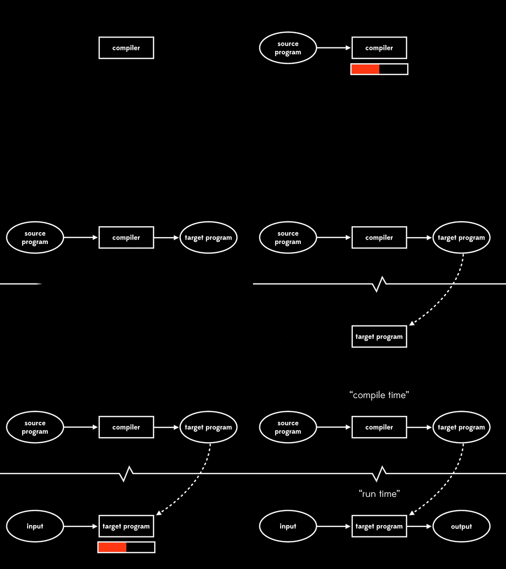
An animation showing a compiler reading a source program to produce a target program, then the target program reading input to produce output

Compilation achieves the same overall result as interpretation — a non-native source program and input are eventually turned into output — but it splits the execution process into two separate stages. The first stage is compile time, when the target program is generated; the second stage is run time, when the input is read and the output is generated.

The good news about compilation is that a good compiler can generate a target program which runs faster than its interpreted counterpart. Splitting the computation into two stages removes the interpretive overhead from run time: all of the work of parsing the program, building an AST and walking over it is done at compile time, so it’s already out of the way by the time the target program runs.

(Incidentally, compilation has other performance benefits too; for example, a compiler can use clever data structures and optimisations to make the target program more efficient, especially if it knows how to exploit the architecture of the underlying machine.)

The bad news about compilation is that it’s just more difficult than interpretation. There are a few reasons for that:

A compiler writer has to think about two stages of execution instead of one. When we write an interpreter, we only need to think about the execution of the interpreter itself and how it’s going to behave at run time in response to the contents of the source program’s AST. But to write a compiler we have to think about both compile time and run time: we must keep track of what the compiler itself is going to do when it generates the target program, and also what the target program will do later when it’s executed.
A compiler writer has to think about two programming languages instead of one. An interpreter is written in a single language, but a compiler contains code written in both the compiler implementation language and the target language — our Simple compiler is written in Ruby interspersed with fragments of JavaScript.
Compiling dynamic languages into efficient target programs is inherently challenging. Languages like Ruby and JavaScript have features which allow the program itself to change and grow during execution, so the static source code of a program doesn’t necessarily tell the compiler everything it wants to know about what might happen at run time.

In short: writing an interpreter is easier than writing a compiler, but interpreted programs are slower than compiled ones. Interpreters only have one execution stage, only use one programming language, and can be as dynamic as necessary — if the program changes when it runs, that’s fine, because the AST can be updated and the interpreter will just keep working — but that ease and flexibility carries a run time performance penalty.

Ideally we would only need to write interpreters for our programming languages, but we want our programs to run as fast as possible, so we usually end up writing compilers wherever possible.

Partial evaluation

Programmers use interpreters and compilers all the time, but there’s another kind of program-manipulating program that’s less well known: partial evaluators. A partial evaluator is a hybrid of an interpreter and a compiler:

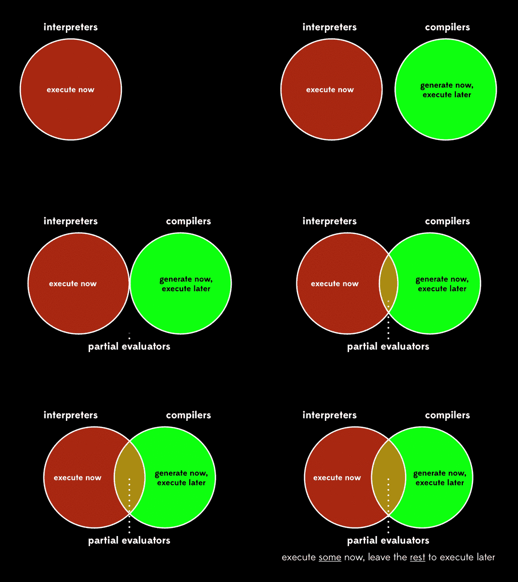
A Venn diagram showing how interpreters (execute now) and compilers (generate now, execute later) overlap to produce partial evaluators (execute some now, leave the rest to execute later)

Whereas an interpreter executes a program right now, and a compiler generates a program now so that we can execute it later, a partial evaluator executes some of the code now and leaves the rest of it for execution later.

A partial evaluator reads a program (called the subject program) along with some of the inputs for that program, and evaluates only the parts of the program that depend on the inputs provided. Once all these parts have been evaluated, the remaining program (called the residual program) is emitted as output.

In this way, partial evaluation lets us extract part of the process of program execution and do it earlier, timeshifting it into the past. Instead of providing all of a program’s inputs at once, we can provide some of them now and save the rest for later.

So, instead of executing the subject program all at once, we can feed it and some of its input into a partial evaluator. The partial evaluator will execute some of the subject program to produce a residual program; later, we can execute the residual program, feeding it the rest of the input to get the final output:

An animation showing a partial evaluator reading a subject program and some of its input to produce a residual program, then the residual program reading the remaining input to produce output

The overall effect of partial evaluation is to split a single-stage execution into two stages by timeshifting some of the work from the future — when we intend to run the program — to the present, so that we can get it out of the way earlier.

A partial evaluator works by turning the subject program into an AST, just like an interpreter or compiler, and reading some of the program’s inputs. It analyses the AST by walking over it to find all the places where the provided inputs are used; each of these program fragments is then evaluated and replaced with new code containing the result. Once partial evaluation is complete, the AST is turned back into text and emitted as the residual program.

That’s too much machinery for us to actually build here, but let’s walk through a manual example to get a feel for what it looks like.

Imagine that some Ruby program contains a method, #power, which calculates x to the power of n:

def power(n, x)
  if n.zero?
    1
  else
    x * power(n - 1, x)
  end
end

Now let’s play the part of a Ruby partial evaluator, and assume that we’ve been given enough of the program’s input to know that #power will be called with 5 as its first argument, n. We can easily generate a new version of the method — let’s call it #power_5 — where the n argument has been removed, and all occurrences of n have been replaced with 5 (this is called constant propagation):

def power_5(x)
  if 5.zero?
    1
  else
    x * power(5 - 1, x)
  end
end

There are now two expressions inside the method — 5.zero? and 5 - 1 — that we could potentially evaluate. Let’s choose to evaluate 5.zero? and replace it with the result, false:

def power_5(x)
  if false
    1
  else
    x * power(5 - 1, x)
  end
end

This change makes it possible to evaluate the whole conditional — if false … else … end always evaluates to the else clause (sparse conditional constant propagation):

def power_5(x)
  x * power(5 - 1, x)
end

Now we can evaluate 5 - 1 and replace it with 4 (constant folding):

def power_5(x)
  x * power(4, x)
end

We could stop there, but because we know the definition of #power, there’s an opportunity to replace the power(4, x) call with the body of #power itself (inline expansion), with the argument 4 replacing all occurrences of the parameter n:

def power_5(x)
  x *
  if 4.zero?
    1
  else
    x * power(4 - 1, x)
  end
end

Now we can just repeat what we did before. We know that 4.zero? evaluates to false:

def power_5(x)
  x *
  if false
    1
  else
    x * power(4 - 1, x)
  end
end

We know that if false … else … end evaluates to the else branch:

def power_5(x)
  x *
  x * power(4 - 1, x)
end

We know that 4 - 1 is 3:

def power_5(x)
  x *
  x * power(3, x)
end

And so on. By repeatedly inlining calls to #power and evaluating constant expressions where possible, we keep adding more multiplications until we get a #power call with 0 as its first argument:

def power_5(x)
  x *
  x *
  x *
  x *
  x * power(0, x)
end

Let’s expand that call:

def power_5(x)
  x *
  x *
  x *
  x *
  x *
  if 0.zero?
    1
  else
    x * power(0 - 1, x)
  end
end

We know that 0.zero? is true:

def power_5(x)
  x *
  x *
  x *
  x *
  x *
  if true
    1
  else
    x * power(0 - 1, x)
  end
end

For the first time we have a conditional that says if true instead of if false. This evaluates to the if branch rather than the else branch:

def power_5(x)
  x *
  x *
  x *
  x *
  x *
  1
end

We’ve ended up with a definition of #power_5 that multiplies x by itself five times and then multiplies by 1. Multiplying a number by 1 doesn’t change it, so let’s eliminate that last multiplication and clean up the formatting to get the finished method:

def power_5(x)
  x * x * x * x * x
end

Here’s what that whole process looks like:

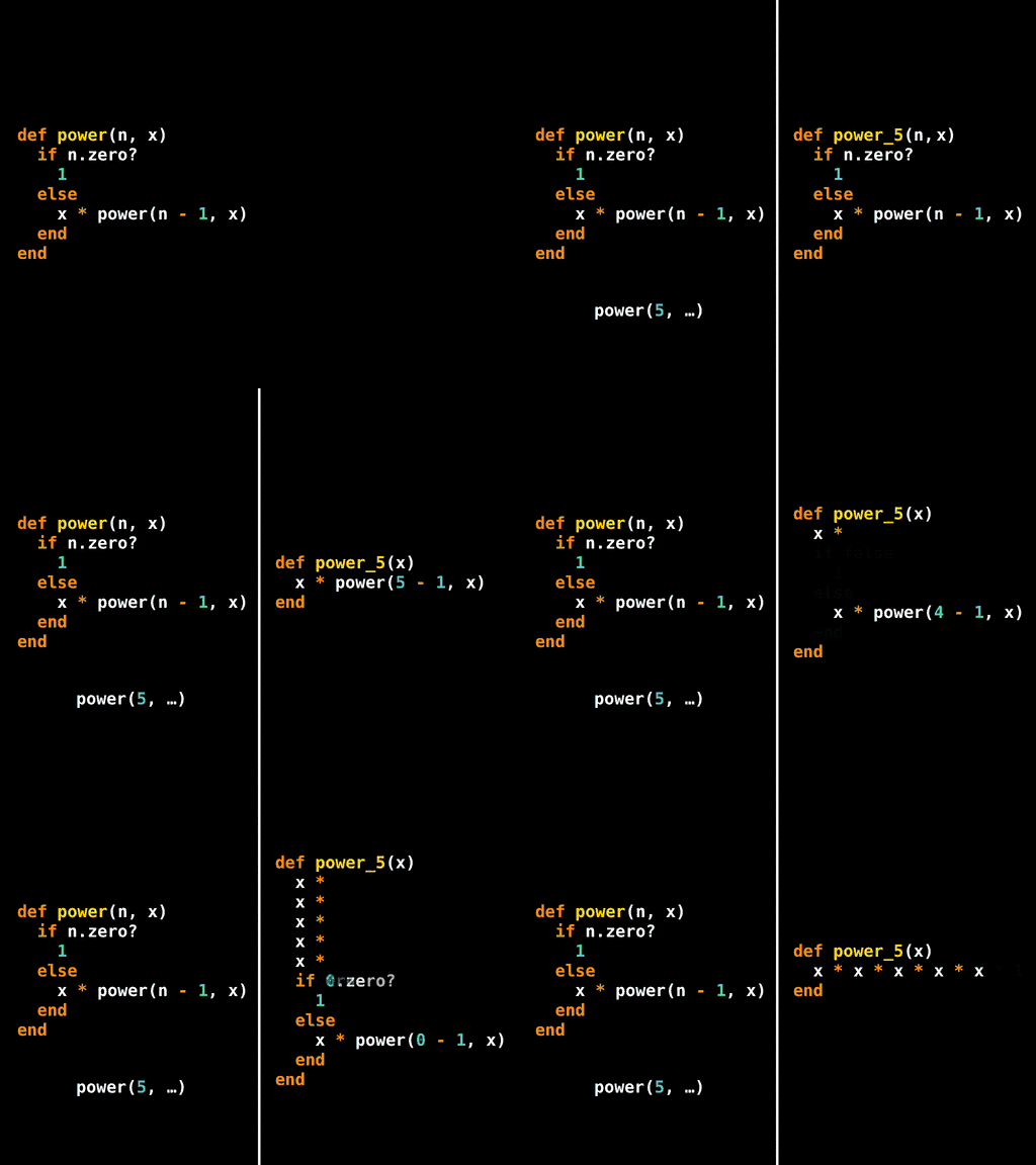
An animation showing how the #power method is partially evaluated to create the #power_5 method

#power_5 is the residual program generated by the partial evaluation of #power with respect to the input 5. There’s no new code in it; #power_5’s body is made up from bits of #power, just rearranged and stuck together in new ways.

The advantage of #power_5 is that it should be faster than #power in the case where n is 5. #power_5 just multiplies x by itself five times, whereas #power executes several recursive method calls, zero checks, conditionals and subtractions. Partial evaluation has done all of that work already, and left behind a residual program which only contains the remaining work that depends on the (unknown) value of x.

So #power_5 is an improved version of #power, if we know that n is going to be 5.

Note that this isn’t the same thing as partial application. We could have used partial application to implement #power_5 differently:

def power_5(x)
  power(5, x)
end

This time we’ve turned #power into #power_5 by simply fixing one of its arguments to a constant value. Of course, this implementation works fine:

>> power_5(2)
=> 32

But this version of #power_5 isn’t any more efficient than #power — if anything it’ll be slightly slower, because it introduces an extra method call.

Or, instead of defining a new method, we could turn #power into a proc with Method#to_proc, use Proc#curry to turn it into a curried proc, and call the curried proc with #power’s first argument (i.e. 5) to partially apply it:

>> power_5 = method(:power).to_proc.curry.call(5)
=> #<Proc (lambda)>

Later, we can call the partially applied proc with #power’s second argument to actually execute the method:

>> power_5.call(2)
=> 32

So, partial application is a bit similar to partial evaluation, but it’s a technique that’s applied inside a program: when we’re writing code, partial application gives us a way to define a lower-arity version of a method by fixing one or more of its arguments. By contrast, partial evaluation is a source-level program transformation that’s applied from outside of a program, generating a faster version of that program by specialising it for particular input values.

Applications

Partial evaluation has many useful applications. The ability to specialise a program for a fixed input can provide the best of both worlds: we can write a general and flexible program that supports many different inputs, and then, when we actually know how we want to use that program, we can use a partial evaluator to automatically generate a specialised version that’s had much of its generality removed to improve its performance.

For example, a web server like nginx or Apache reads in a configuration file when it starts up. The contents of that file affect the handling of every HTTP request, so the web server must spend some of its execution time checking its configuration data to decide what to do. If we used a partial evaluator to specialise a web server with respect to a particular config file, we’d get a new version that only does what that file says; the overhead of parsing a config file during startup, and checking its data during every request, would no longer be part of the program.

Another classic example is ray tracing. To make a movie where the camera moves through a three-dimensional scene, we might end up using a ray tracer to render thousands of individual frames. But if the scene’s the same for every frame, we could use a partial evaluator to specialise the ray tracer with respect to our particular scene description, and we’d get a new ray tracer that could only render that scene. Then, each time we used the specialised ray tracer to render a frame, we’d avoid the overhead of reading the scene file, setting up the data structures needed to represent its geometry, and making camera-independent decisions about how rays of light behave in the scene.

A more practical (although more questionable) example is the OpenGL pipeline. In OS X, parts of the OpenGL pipeline are written in LLVM intermediate language, including functionality which is implemented directly in hardware on some GPUs. By shipping software implementations of features that any particular GPU may or may not have, Apple makes it possible for LLVM to partially evaluate away any unnecessary code when it’s run on specific hardware, with any hardware-unsupported features being provided by the residual software.

The Futamura projections

At the beginning I said I’d tell you a cool story, so here it is.

In 1971, Yoshihiko Futamura realised something interesting while he was working at Hitachi Central Research Laboratory. He was thinking about how partial evaluation allows us to process some of a subject program’s input earlier, leaving us with a residual program that we can run later.

Specifically, Futamura was thinking about partial evaluation in the context of interpreters. He realised that an interpreter is just a computer program that we provide with inputs and then execute to produce output. One of its inputs happens to be source code, but otherwise an interpreter is like any other program that turns inputs into output.

What would happen, he wondered, if we used partial evaluation to do some of an interpreter’s work earlier, and do the rest of it later by running the residual program?

If we use partial evaluation to specialise an interpreter with respect to one of its inputs — a particular source program — we get a residual program out. Then, at some later time, we can run that residual program with the remaining input to get the final output:

An animation showing a partial evaluator reading an interpreter and a source program to produce a residual program, then the residual program reading input to produce output

The overall effect is the same as running the interpreter directly against the source program and its input, but now that execution has been split into two stages.

Futamura noticed that this residual program, which reads in the final input and produces output, is what we’d usually call a target program — a version of the source program that can be executed directly on the underlying machine. That means that the partial evaluator has read in a source program and produced a target program; in other words, it’s acted as a compiler.

An animation identifying the residual program as a target program, indicating that the partial evaluator has acted as a compiler

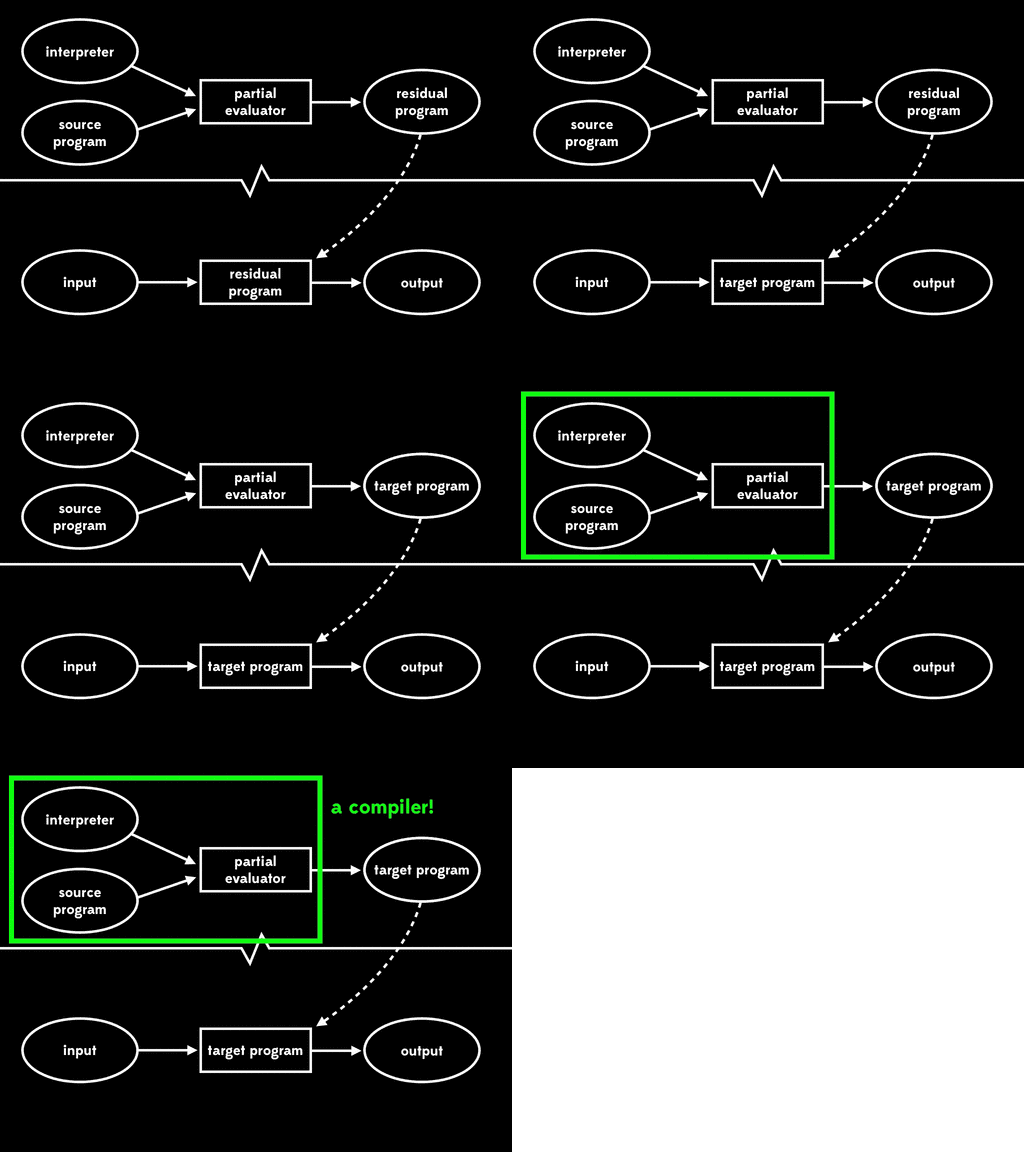
That’s pretty amazing. How does it work? Let’s work through a quick example.

Here’s the top level of a Simple interpreter written in Ruby:

source, environment = read_source, read_environment

Treetop.load('simple.treetop')
ast = SimpleParser.new.parse(source).to_ast
puts ast.evaluate(environment)

This interpreter reads in the source program and its initial environment from somewhere (we don’t care how). It loads the Treetop grammar, instantiates the parser, and uses it to turn the source into an AST. Then it evaluates the AST and prints out the environment so we can see the final values of all the variables. The definitions of #evaluate on each kind of AST node aren’t shown here — they’re the same as before.

Let’s imagine feeding this interpreter into a Ruby partial evaluator with a particular Simple source program, x = 2; y = x * 3, as input. That means #read_source (however it works) will return the string 'x = 2; y = x * 3', so we can replace the read_source call with that value:

source, environment = 'x = 2; y = x * 3', read_environment

Treetop.load('simple.treetop')
ast = SimpleParser.new.parse(source).to_ast
puts ast.evaluate(environment)

Now we can do some copy propagation; the source variable is only used once, so we can eliminate it entirely and replace it with its value:

environment = read_environment

Treetop.load('simple.treetop')
ast = SimpleParser.new.parse('x = 2; y = x * 3').to_ast
puts ast.evaluate(environment)

This gives us all the data necessary to built the AST; we already have the Treetop grammar, and now we know what string we’re going to parse with it. Let’s evaluate the expression that creates the AST and replace it with the AST itself:

environment = read_environment

ast = Sequence.new(
        Assign.new(
          :x,
          Number.new(2)
        ),
        Assign.new(
          :y,
          Multiply.new(
            Variable.new(:x),
            Number.new(3)
          )
        )
      )
puts ast.evaluate(environment)

At this point we’ve reduced the general Simple interpreter to a program which reads in an environment, constructs a literal AST, and calls #evaluate on it.

What does calling #evaluate on this specific AST do? Well, we already have the definitions of #evaluate for each kind of AST node, so we can walk over the tree and partially evaluate each occurrence of #evaluate, just as we did for #power. The AST contains all the data we need, so we can gradually boil down all of these #evaluate implementations to a couple of lines of Ruby:

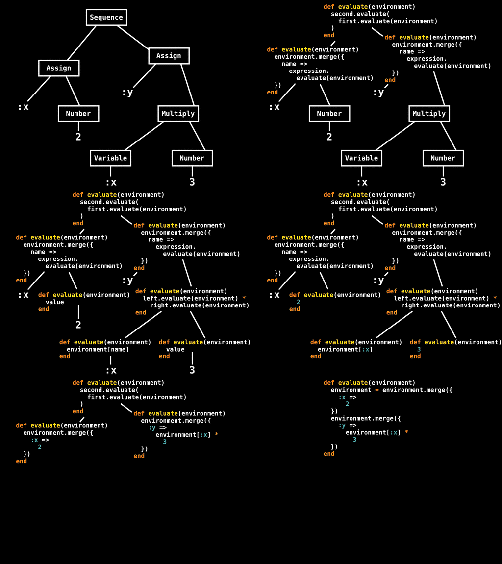
An animation showing how the #evaluate method is partially evaluated across each node of the AST

For the Number and Variable leaves we know what the values of value and name are, so we can propagate those constants into the definitions of #evaluate for those nodes. For the Multiply and Assign nodes that evaluate their subexpressions, we can inline the recursive #evaluate calls by looking at the appropriate method definitions. And for the Sequence node, we can inline the calls to first.evaluate and second.evaluate, using a temporary variable to hold the value of the intermediate environment.

That glosses over a tremendous amount of detail, but the important thing is that we have all of the code and data we need to build a partially-evaluated definition of #evaluate for the root node of the AST:

def evaluate(environment)
  environment = environment.merge({ :x => 2 })
  environment.merge({ :y => environment[:x] * 3 })
end

Let’s go back to the main interpreter code:

environment = read_environment

ast = Sequence.new(
        Assign.new(
          :x,
          Number.new(2)
        ),
        Assign.new(
          :y,
          Multiply.new(
            Variable.new(:x),
            Number.new(3)
          )
        )
      )
puts ast.evaluate(environment)

Now that we’ve generated the body of #evaluate for the AST’s root node, we can partially evaluate ast.evaluate(environment) by expanding the #evaluate call:

environment = read_environment

environment = environment.merge({ :x => 2 })
puts environment.merge({ :y => environment[:x] * 3 })

This is a Ruby program that reproduces the behaviour of the original Simple program: it sets x to 2 in the environment, then sets y to the value of x multiplied by 3. So, in a sense, we’ve compiled the Simple program into Ruby by partially evaluating an interpreter — there’s some extra machinery involving the environment, but what we’ve ended up with is essentially a Ruby version of x = 2; y = x * 3.

As with the #power example, we didn’t have to write any new Ruby code; the residual program is just pieces of the interpreter rearranged and stuck together in such a way that it does the same thing as the Simple program we started with.

This is called the first Futamura projection: if we partially evaluate an interpreter with respect to some source code, we get a target program.

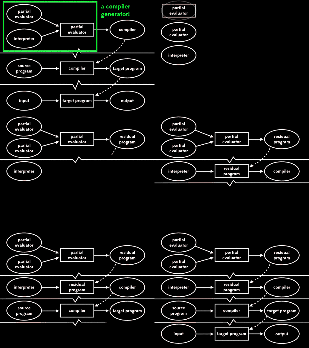
Futamura was happy when he realised this. Then he thought about it some more, and realised that when we feed an interpreter and a source program into the partial evaluator to produce a target program, this is just another instance of running a program with multiple inputs. What would happen if we used partial evaluation to do some of the partial evaluator’s work earlier, and do the rest of it later by running the residual program?

If we use partial evaluation to specialise the partial evaluator with respect to one of its inputs — the interpreter — we get a residual program out. Then, at some later time, we can run that residual program with the source program as input to get a target program. And lastly, we can run the target program with the remaining input to get the final output:

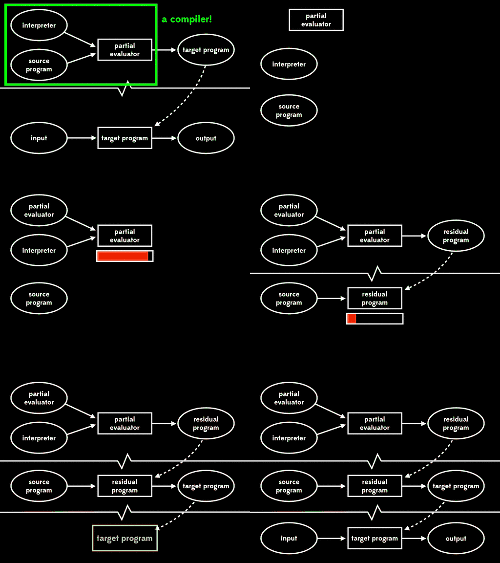
An animation showing a partial evaluator reading a partial evaluator and an interpreter to produce a residual program, then the residual program reading a source program to produce a target program, then the target program reading input to produce output

The overall effect is the same as running the interpreter directly against the source program and its input, but now that execution has been split into three stages.

Futamura noticed that this residual program, which reads in the source program and produces a target program, is what we’d usually call a compiler. That means that the partial evaluator has read in an interpreter and produced a compiler; in other words, it’s acted as a compiler generator.

An animation identifying the residual program as a compiler, indicating that the partial evaluator has acted as a compiler generator

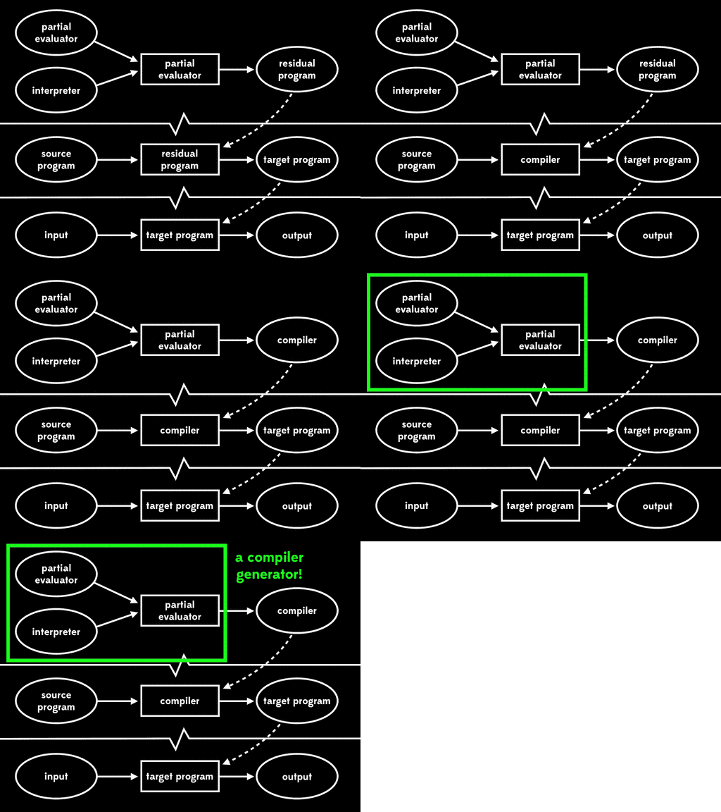
This is called the second Futamura projection: if we partially evaluate a partial evaluator with respect to an interpreter, we get a compiler.

Futamura was happy when he realised this. Then he thought about it some more, and realised that when we feed a partial evaluator and an interpreter into the partial evaluator to produce a compiler, this is just another instance of running a program with multiple inputs. What would happen if we used partial evaluation to do some of the partial evaluator’s work earlier, and do the rest of it later by running the residual program?

If we use partial evaluation to specialise the partial evaluator with respect to one of its inputs — the partial evaluator — we get a residual program out. Then, at some later time, we can run that residual program with the interpreter as input to get a compiler. Later still, we can run the compiler with the source program as input to get a target program. And lastly, we can run the target program with the remaining input to get the final output:

An animation showing a partial evaluator reading a partial evaluator and a partial evaluator to produce a residual program, then the residual program reading an interpreter to produce a compiler, then the compiler reading a source program to produce a target program, then the target program reading input to produce output

The overall effect is the same as running the interpreter directly against the source program and its input, but now that execution has been split into four stages.

Futamura noticed that this residual program, which reads in the interpreter and produces a compiler, is what we’d usually call a compiler generator. That means that the partial evaluator has produced a compiler generator; in other words, it’s acted as a compiler generator generator.

An animation identifying the residual program as a compiler generator, indicating that the partial evaluator has acted as a compiler generator generator

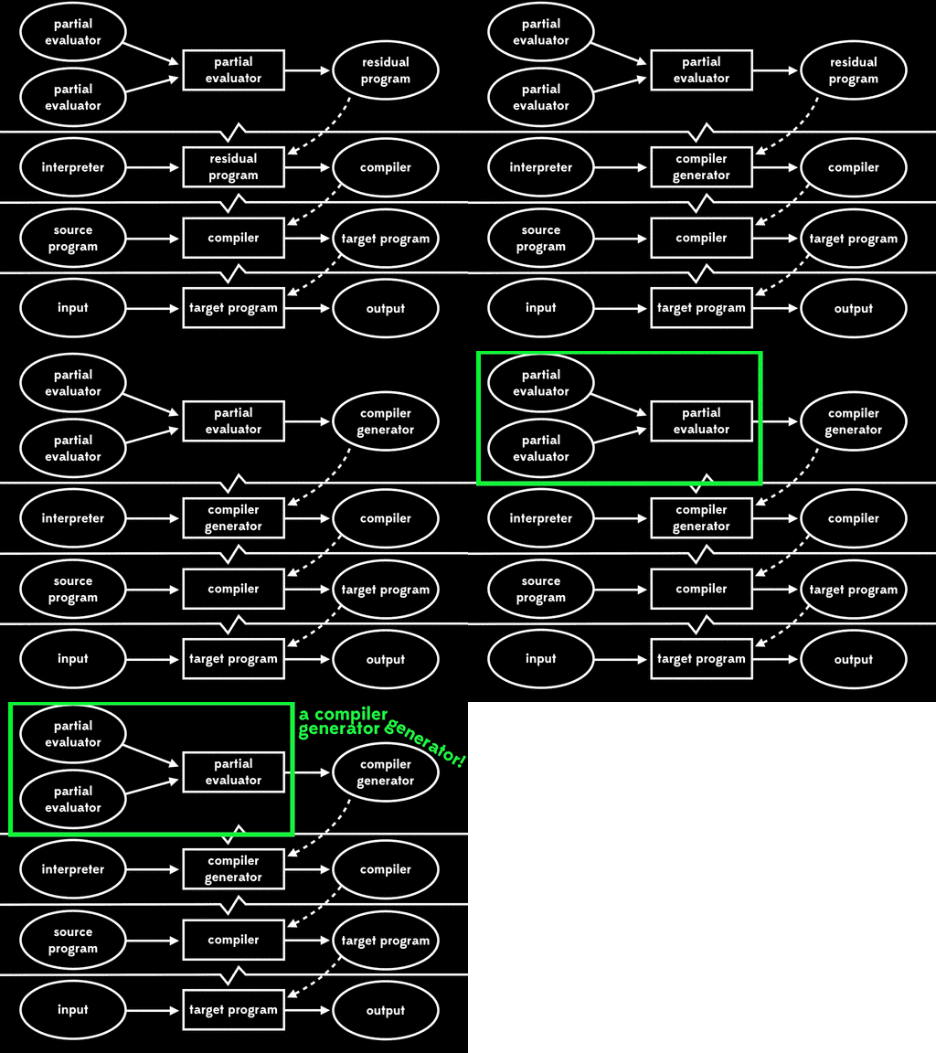
This is the third Futamura projection: if we partially evaluate a partial evaluator with respect to a partial evaluator, we get a compiler generator.

Thankfully we can’t take it any further than that, because if we repeated the process we’d still be partially evaluating the partial evaluator with respect to itself. There are only three Futamura projections.

Conclusion

The Futamura projections are fun and surprising, but their existence doesn’t make compiler authors redundant. Partial evaluation is a fully general technique that works with any computer program; when applied to an interpreter it can eliminate the overhead of parsing source code and manipulating an AST, but it doesn’t spontaneously invent the kind of data structures and optimisations that we expect from a production-quality compiler. We still need clever people to hand-craft compilers to make our programs go as fast as possible.

If you’d like to learn more about partial evaluation, there’s a great free book called “Partial Evaluation and Automatic Program Generation” that explains it in detail. The JIT in LLVM, and parts of the PyPy toolchain — namely RPython and the VM and the JIT that underlie it — use related techniques to execute programs efficiently. Those projects are directly relevant to Ruby because Rubinius sits on top of LLVM, and there’s a Ruby implementation written in Python, called Topaz, that sits on top of the PyPy toolchain.

Partial evaluation aside, Rubinius and JRuby are high-quality compilers with interesting and accessible implementations. If you’re interested in programs that manipulate programs, you may enjoy cracking open Rubinius or JRuby, having a look at how they work, and (in the spirit of Matz’s RubyConf 2013 keynote) getting involved in their development.

Contents