Hello, declarative world
Contents
Introduction
I recently read a good rant in an article called “Can Programming Be Liberated from the von Neumann Style?”. The term “von Neumann style” refers to programming languages whose design reflects the way a computer actually works: they have variables to represent memory locations, assignment statements to write to those locations, loops and branches to control the program counter, and so on.
These languages encourage us to do what Bret Victor calls “playing computer” — spending a lot of time thinking about how computers work, and adapting our ideas to compensate. The article is an angry explanation of why this is a terribly restrictive way of writing programs, and a call to think more broadly and creatively about how we can express ideas as code.
I found it very persuasive, but unfortunately the rant was written in 1978, by John Backus, the designer of FORTRAN. John Backus died in 2007, and a lot of his complaints are still valid today. So his rant wasn’t a total success; it was influential, but perhaps not as much as it could have been. We’re still stuck with mostly “von Neumann style” languages that talk about state and assignment and memory and stuff — computer things, not idea things.
I want to continue that rant and ask you to consider the possibility of finding different ways of explaining ourselves to computers.
Programming paradigms
I’ll begin by briefly mentioning a few different programming paradigms. The first is unstructured programming. An example of unstructured programming is assembly language: programs consist of a linear sequence of instructions interrupted by the occasional jump. A programmer in an unstructured language can ask the computer to perform one instruction after another, and to conditionally go to a different place in the program.
Slightly better than unstructured languages are procedural languages, which let you jump into a part of the program, do some work, and then jump back to wherever you came from. Those jumps can be nested so that procedures can call other procedures, which is a definite improvement upon just having a flat sequence of instructions.
Better still are functional languages, which introduce the idea of first-class functions: procedures become values which can travel around your program like any other data.
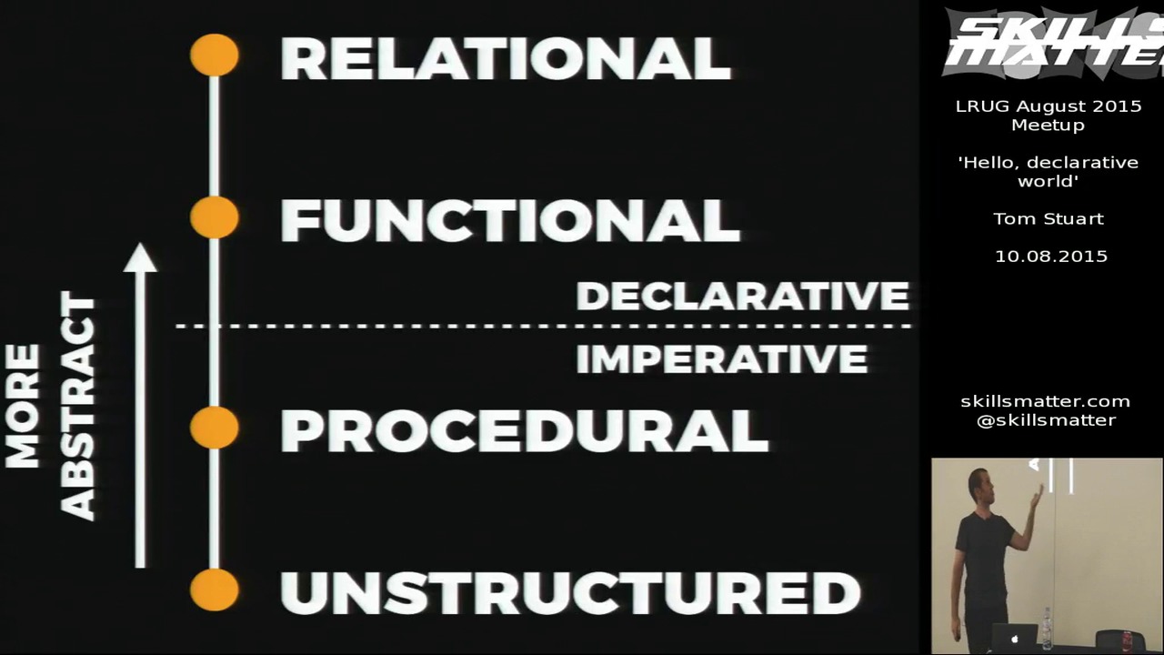
We can arrange those paradigms in roughly increasing order of abstraction. At the bottom is unstructured programming, because it’s as close as we can get to the bare metal of the computer. As we get higher up, our programming languages start being less about how computers work and more about how humans think about problems.
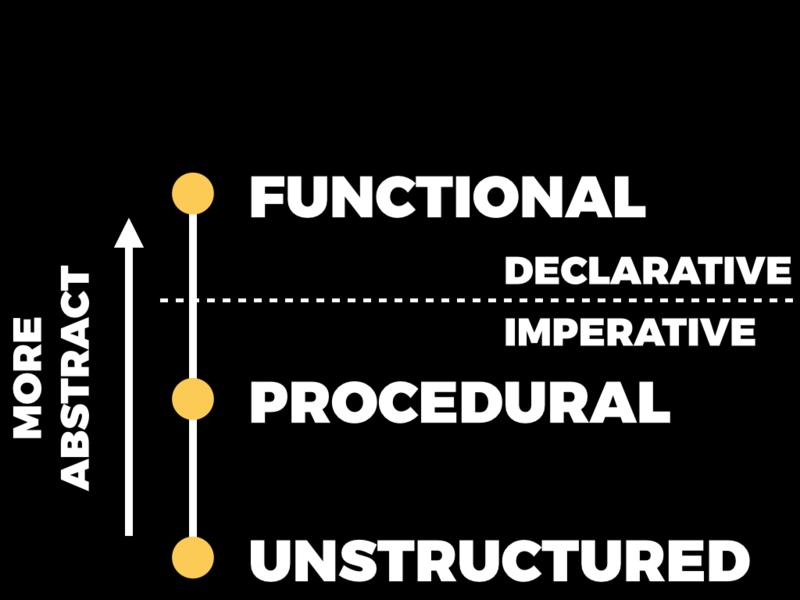
The paradigms separate roughly into imperative and declarative styles. The imperative style is what we would probably all consider to be “normal” programming: that’s where the programmer is responsible for providing these low-level instructions about how a problem should be solved.
By contrast, declarative languages divide the responsibility more evenly between the user and the machine. In these systems it’s the programmer’s job to describe a problem, or a goal, or a set of constraints, which is really the job of saying what needs to be done; then they pass that description over to a solver, which is usually just a conventional imperative program, and it’s the solver’s job to decide how to achieve what the programmer has described.
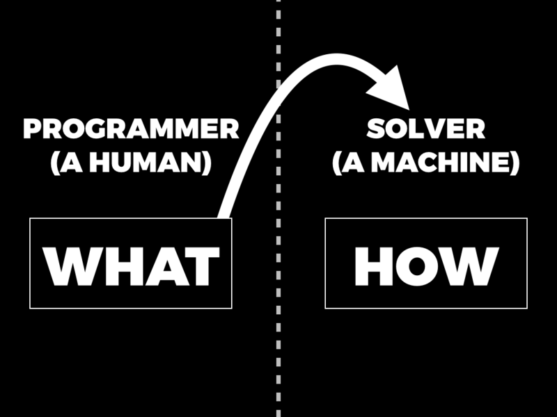
This is a useful division of responsibility because the solver might be able to do a much better job of working out how to do something than a human would. Often there are ways of solving problems that aren’t obvious to humans, and a solver can package up a lot of specialised ingenuity about how to solve particular kinds of problem, and apply it to whatever problem the programmer has described. That lets the programmer focus on describing problems accurately and completely, instead of coming up with lists of fiddly instructions for the computer to follow.
Functional programs tend to live in the declarative world to some degree. Because they generally don’t rely on mutable state, they allow the solver — the language’s runtime, or compiler, or whatever — to have more freedom to decide what order evaluation should happen in, or whether work can be done lazily, or done in parallel, and so on.
We can extend the continuum of abstraction a step further by introducing relational programming.
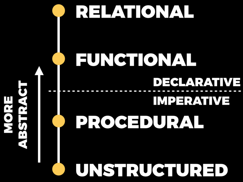
That’s what this article is about: how relational programming takes functional programming to the next level.
Functions and relations
Let’s briefly recap some basics. In functional programming, a function is a black box that has some inputs and an output. You run a function by providing it with some input values and then, when you execute the function, you get an output value back out.
Now, in a functional language, internally a function is specified by some kind of rule which explains how to create the output from the inputs. The function below has a simple underlying rule: if the inputs are called x and y, then the output is x + y.
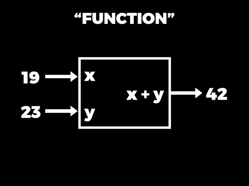
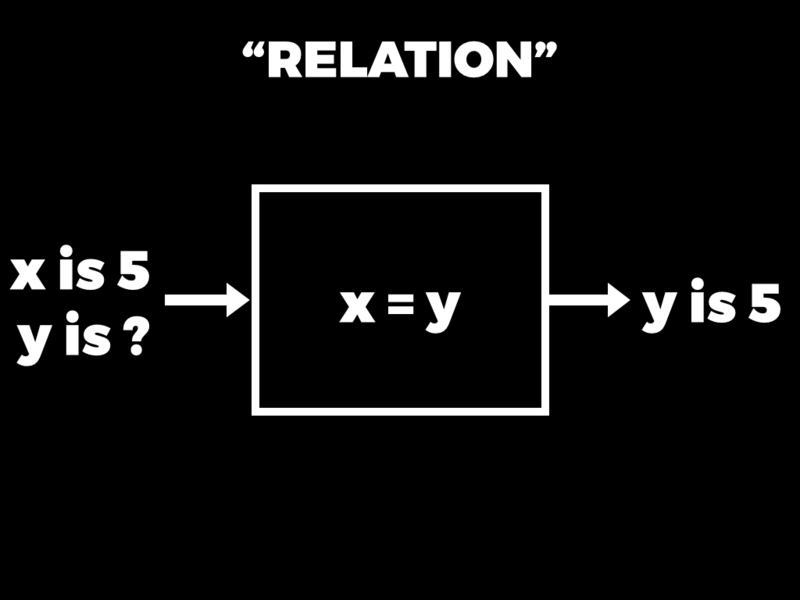
This whole notion of a function as a rule that can be executed to turn inputs into output feels very natural to us, but only because it’s what we’re used to. In both mathematics and programming, a function is a special case of a more general idea called a relation. A relation also has a rule inside it, but the rule is a constraint like x = y. That’s not something that you can run like a function — it doesn’t have inputs or outputs — but what you can do is query the relation that’s defined by the rule.
So we could ask, for example: if x is 5, what can y be? And the answer is: oh, in that case, y is 5.
Or we could have a different rule, like x < y. And then we could ask: if y is 5, what can x be? And the answer comes back: well, x could be 4, or 3, or 2, or 1, or 0. There are many possible answers in that case.
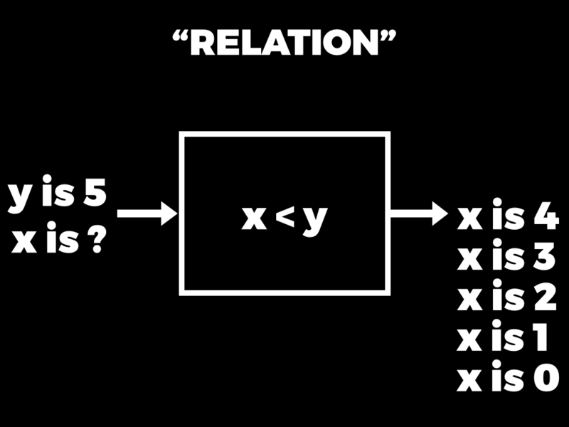
This is essentially what relational programming languages let us do. We can establish rules that relate variables to each other, and then can ask questions about the values of those variables in different situations.
That might seem like a pretty alien idea, but it does show up in more familiar contexts. SQL, for example, is a language which allows us to query a relation, but the rule of that relation is usually specified as a table of data on disk. Different queries of the same table can treat different columns of that table as being inputs or outputs depending on what kind of question we ask.
A relational programming language is kind of like that, but instead of a finite table of data stored on disk, a relations can be defined by a programmatic rule, just like a function can be in a functional language. So we can write these programmatic relations in a relational language, and then instead of running a function to turn input values into output values, we can query a relation to turn the values of some variables into the possible values of other variables.
Building a relational language
To make these rough ideas more precise, I’m going to show you how we can build a little relational language inside Ruby. Of course Ruby isn’t actually relational, so we can’t just make a relation and have it work natively. Instead we’ll design some Ruby objects which allow us to solve problems in a more relational style. That’ll give us some of the flavour of relational programming without having to learn (or invent) a whole new language.
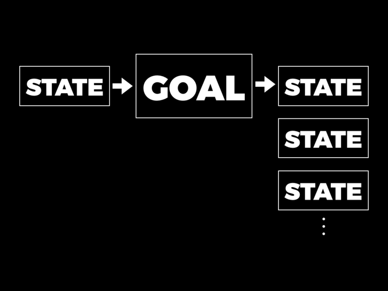
Here’s the big-picture view of how the little relational language works. The programmer’s job is to build a structure called a goal out of Ruby primitives that we provide. A goal contains a rule that places constraints on the values of variables; in this simple language these will just be equality constraints like “x = y” or “z = 4”.
Once a goal has been built, the programmer can ask the computer to pursue the goal in a particular input state. (A state is just a collection of variables and their values.) When a goal is pursued in a particular state, the programmer gets back a stream of output states that satisfy that goal. There might be zero states if the goal can’t be satisfied.
Variables
Our little relational language has first-class variables, just like functional languages have first-class functions. In most languages a variable is only a convenient name for a value, but in relational languages a variable is something concrete that you can explicitly pass around a program like any other value.
The first thing we need to implement, then, is a concrete representation of variables. How should they work?
The only real requirement is that each variable has a unique identity. If we make two separate variables called x and y…
>> x, y = Variable.new(:x), Variable.new(:y)
=> [x, y]
…we want the variable x to be equal to itself…
>> x == x
=> true
…and we want for two different variables, x and y, to not be equal:
>> x == y
=> false
We want this behaviour even if two variables happen to have the same name. If we compare a variable called x to another variable called x, we should still be able to tell that they’re different variables:
>> x == Variable.new(:x)
=> false
This highlights the fact that variable names have no real meaning, and are just there for convenience and readability. A variable’s name is not guaranteed to be unique, and isn’t part of the identity of the variable.
We can get all this behaviour by introducing a Variable class that doesn’t have any interesting operations at all:
class Variable
  def initialize(name)
    @name = name
  end

  def inspect
    @name
  end
end
Each variable will be a unique instance of this Variable class, and variable equality will be decided by object identity. The name of a variable only affects what it looks like when inspected in IRB.
States
Once we have variables, we can package them up into states, which associate variables with possible values. This is what states look like:
class State
  def initialize(variables = [], values = {})
    @variables, @values = variables, values
  end
end
A state contains an array of all the variables that exist and a hash of what values some of those variables have been assigned. (A “value” here means anything that can be compared for equality — in our case, any Ruby value. Our little language doesn’t care about the structure of values, only that they can be compared for equality.)
We’ll give our states some getters so that we can easily look inside and see what variables have been declared and what values, if any, they have:
class State
  attr_reader :variables, :values
end
States are immutable, so they don’t need setters, but they do need two basic operations: we must be able to declare new variables inside a state, and we must be able to assign values to those variables.
Declaring new variables should work like this:
>>state = State.new=> #<State @variables=[], @values={}> >>state, (x, y, z) = state.create_variables [:x, :y, :z]=> [#<State @variables=[x, y, z], @values={}>, [x, y, z]] >>state.variables=> [x, y, z]
#create_variables returns two things: a new state where those variables have been declared, and the new variables themselves. (We can assign each new variable to a separate Ruby variable by using destructuring assignment.) Note that #create_variables doesn’t change the original state — it just returns a new one.
Here’s how assigning values to variables should work:
>>state = state.assign_values x => y, y => z, z => 5=> #<State @variables=[x, y, z], @values={x=>y, y=>z, z=>5}> >>state.values=> {x=>y, y=>z, z=>5}
The above code uses #assign_values to assign y to x, and z to y, and 5 to z, which returns a new state that remembers all those assignments.
The new state knows that x’s value is whatever y is, and y’s value is whatever z is, and z’s value is 5. That kind of means that x’s value is 5, but the state only indirectly records that information.
The actual implementations of #create_variables and #assign_values are straightforward:
class State
  def create_variables(names)
    new_variables = names.map { |name| Variable.new(name) }

    [
      State.new(variables + new_variables, values),
      new_variables
    ]
  end

  def assign_values(new_values)
    State.new(variables, values.merge(new_values))
  end
end
#create_variables instantiates some new variables and adds them to the array of declared variables, and #assign_values merges the new assignments with the existing assignments. There’s nothing interesting going on.
So, those are the two ways that a state develops over time: #create_variables grows the collection of declared variables, and #assign_values grows the collection of values assigned to them.
Since variables can be assigned to other variables, it’s helpful to have an operation called #value_of that can find the ultimate value of a variable:
>> state.value_of x
=> 5
#value_of lets us ask for the value of x and get the answer 5 by repeatedly traversing variable assignments.
Asking for the value of anything that’s not an assigned variable just returns that value:
>> state.value_of 7
=> 7
That’s even the case if we ask for the value of a variable that hasn’t been assigned yet:
>>state, (a, b, c) = state.create_variables [:a, :b, :c]=> [#<State …>, [a, b, c]] >>state.value_of a=> a
The value of a is just a again, because a hasn’t had anything assigned to it.
Here’s how to implement #value_of:
class State
  def value_of(key)
    if values.has_key?(key)
      value_of values.fetch(key)
    else
      key
    end
  end
end
This implementation recursively looks up a value in a state. If a value has an assignment in the values hash, #value_of retrieves its assigned value, and then tries to look that up. That process repeats until it reaches a value with no assignment and returns it.
Unification
Now that we’ve built variables and states, we can move on to implementing unification, which is the workhorse of this little language. Unification is the process of making two values equal in a particular state, and it works by adding assignments to that state.
Here’s an example. If we start with an empty state, give it two variables x and y, and then try to unify x with itself in that state, then unification should succeed and return the same state:
>>state = State.new=> #<State @variables=[], @values={}> >>state, (x, y) = state.create_variables [:x, :y]=> [#<State @variables=[x, y], @values={}>, [x, y]] >>state = state.unify(x, x)=> #<State @variables=[x, y], @values={}> >>state.values=> {}
No changes are required to make x and x equal, because they’re already equal, so unification does nothing and we get the original state back.
If we unify two different variables — for example, if we try to make x equal to y — then we should get back a state that makes them equal:
>>state = state.unify(x, y)=> #<State @variables=[x, y], @values={x=>y}> >>state.values=> {x=>y} >>state.value_of x=> y
Unification has made x and y equal by adding an assignment to the state — x now has the value y.
If we then try to unify x with some other value, like 5, here’s what happens:
>>state = state.unify(x, 5)=> #<State @variables=[x, y], @values={x=>y, y=>5}> >>state.values=> {x=>y, y=>5}
x had already been assigned the value y, so unification has made x equal to 5 by adding an assignment that says y is 5.
If we ask again for the value of x, we’ll see that it’s now 5 as requested:
>> state.value_of x
=> 5
If we try to make either variable equal to a different value — for example, if we try to make y equal to 6 — then unification will return nil to indicate failure:
>> state.unify(y, 6)
=> nil
This happens because x and y are already both equal to 5, so there’s no way to make y be 6 without undoing some of the existing assignments.
The implementation of #unify is surprisingly simple:
class State
  def unify(a, b)
    a, b = value_of(a), value_of(b)

    if a == b
      self
    elsif a.is_a?(Variable)
      assign_values a => b
    elsif b.is_a?(Variable)
      assign_values b => a
    end
  end
end
To make its two arguments equal, #unify first uses #value_of to find their final values in the current state. If those values are already equal then it returns the current state; otherwise, if either value is a variable, #unify adds an assignment to the state to make that variable equal to the other value. If neither value is a variable, it falls off the end of the if-elsif expression and returns nil to indicate failure.
Goals
Now we’re ready to introduce goals and the operations that build them. Every goal will be an instance of this class:
class Goal
  def initialize(&block)
    @block = block
  end

  def pursue_in(state)
    @block.call state
  end
end
A goal simply wraps up a block of code, and to pursue that goal in a particular state, the block is called with the state as an argument. So “goal” is really just a nice name for a Proc, but having a dedicated Goal class gives us somewhere convenient to put methods for building different kinds of goal.
Basic goals
There are only four kinds of goal in the language we’re building, and two of them are very basic.
The first kind, called equal, is the only kind of goal that isn’t made out of other goals. An equal goal contains two values, and when it’s pursued in a particular state, it tries to make its two values equal by unifying them in that state.
Here’s an example. We’ll make a new state that has some variables in it, and then use a Goal.equal factory method to make a goal that says x is equal to 5:
>>state = State.new=> #<State @variables=[], @values={}> >>state, (x, y, z) = state.create_variables [:x, :y, :z]=> [#<State @variables=[x, y, z], @values={}>, [x, y, z]] >>goal = Goal.equal(x, 5)=> #<Goal @block=#<Proc>>
If we pursue that goal in our original empty state, we get back a stream of results:
>> states = goal.pursue_in(state)
=> #<Enumerator: #<Enumerator::Generator>:each>
(We’re using an enumerator to represent a stream here. An enumerator is just an object we can call #next on and keep getting more values out.)
The first result in the stream is a state that says the value of x is 5:
>>state = states.next=> #<State @variables=[x, y, z], @values={x=>5}> >>state.values=> {x=>5} >>state.value_of x=> 5
So the goal has succeeded in making x equal to 5.
If we try to retrieve another result from the stream we get a StopIteration exception, because the goal only produced one state:
>> states.next
StopIteration: iteration reached an end
Here’s how Goal.equal is implemented:
def Goal.equal(a, b)
  Goal.new do |state|
    state = state.unify(a, b)

    Enumerator.new do |yielder|
      yielder.yield state if state
    end
  end
end
To construct an equal goal we have to provide the two values, a and b. When the goal is pursued in a particular state, it unifies a and b in that state and produces a stream of states — an enumerator — as its result.
The code inside the Enumerator.new block yields an output state if unification was successful, otherwise it does nothing, so the resulting stream either contains a single state or is empty.
Explicitly creating variables just to pass them to a goal is a bit inconvenient, which is why we have the other kind of basic goal, called with_variables. The job of a with_variables goal is to run an existing goal and automatically provide it with as many local variables as it needs.
For example, we can take an equal goal that expects to use a variable called x, and wrap it up into a with_variables goal so that the local variable x is automatically created when we need it:
>>goal = Goal.with_variables { |x| Goal.equal(x, 5) }=> #<Goal @block=#<Proc>> >>states = goal.pursue_in(State.new)=> #<Enumerator: #<Enumerator::Generator>:each> >>state = states.first=> #<State @variables=[x], @values={x=>5}> >>state.values=> {x=>5}
This time we didn’t have to create the variable x ourselves — when we pursue the goal and inspect the resulting states, we can see that it’s been created for us.
This is pretty easy to implement in Ruby because we can examine a block with Proc#parameters:
def Goal.with_variables(&block)
  names = block.parameters.map { |type, name| name }

  Goal.new do |state|
    state, variables = state.create_variables(names)
    goal = block.call(*variables)
    goal.pursue_in state
  end
end
We can call Goal.with_variables with a block and get back a goal. When that goal is pursued, it automatically creates the right number of variables for our block, calls it with them, and pursues whatever goal is returned.
Combining goals
So those are the two basic goals: making values equal, and introducing local variables automatically. There are two other kinds of combining goal that we can use to plug together the basic goals to make larger and more interesting ones.
The first combining goal is called either. It combines two goals by pursuing each of them independently and combining their output streams. Every output state from an either goal satisfies either its first or its second subgoal.
Here’s an example of that. We want to be able to say either x equals 5, or x equals 6:
>> goal = Goal.with_variables { |x|
     Goal.either(
       Goal.equal(x, 5),
       Goal.equal(x, 6)
     )
   }
=> #<Goal @block=#<Proc>>
When we pursue that goal in an empty state, the stream we get back has two result states in it:
>>states = goal.pursue_in(State.new)=> #<Enumerator: #<Enumerator::Generator>:each> >>states.next.values=> {x=>5} >>states.next.values=> {x=>6}
One of them says that x is 5, and the other one says x is 6.
The implementation of Goal.either is very short:
def Goal.either(first_goal, second_goal)
  Goal.new do |state|
    first_stream = first_goal.pursue_in(state)
    second_stream = second_goal.pursue_in(state)

    first_stream.interleave_with(second_stream)
  end
end
It pursues each goal separately, then combines the resulting streams by interleaving them. Unfortunately, there is no Enumerator#interleave_with method in Ruby, so we have to implement that too.
We should be able to interleave, say, a stream of letters and a stream of numbers to get a stream of both letters and numbers:
>>letters = 'a'.upto('z')=> #<Enumerator: "a":upto("z")> >>numbers = 1.upto(10)=> #<Enumerator: 1:upto(10)> >>letters.interleave_with(numbers).entries=> ["a", 1, "b", 2, "c", 3, "d", 4, "e", 5, "f", 6, "g", 7, "h", 8, "i", 9, "j", 10, "k", "l", "m", "n", "o", "p", "q", "r", "s", "t", "u", "v", "w", "x", "y", "z"]
Notice that we get a letter, then a number, then another letter, then another number and so on, and when the numbers run out we just get the rest of the letters.
It would be helpful if this worked even when the streams are infinite. So if we have an infinite stream of the letters 'a', 'b' and 'c' repeating over and over, and an infinite stream of the numbers from 1 up to infinity, we should still be able to interleave them:
>>letters = ['a', 'b', 'c'].cycle=> #<Enumerator: ["a", "b", "c"]:cycle> >>numbers = 1.upto(Float::INFINITY)=> #<Enumerator: 1:upto(Infinity)> >>letters.interleave_with(numbers).take(50)=> ["a", 1, "b", 2, "c", 3, "a", 4, "b", 5, "c", 6, "a", 7, "b", 8, "c", 9, "a", 10, "b", 11, "c", 12, "a", 13, "b", 14, "c", 15, "a", 16, "b", 17, "c", 18, "a", 19, "b", 20, "c", 21, "a", 22, "b", 23, "c", 24, "a", 25]
Here’s how to implement it:
class Enumerator
  def interleave_with(other)
    enumerators = self, other

    Enumerator.new do |yielder|
      until enumerators.empty?
        loop do
          enumerator = enumerators.shift
          yielder.yield enumerator.next
          enumerators.push enumerator
        end
      end
    end
  end
end
The inner loop of this implementation bounces back and forth between the two enumerators until they’ve both finished. It relies on Enumerator#next raising a StopIteration exception when each stream runs out, which breaks out of the inner loop and discards the finished stream. If either enumerator is infinite it just keeps going forever.
The other combining goal is called both. It’s slightly more complicated.
It combines two goals by pursuing the first goal to get a stream of states, then pursuing the second goal in each of those states and combining the many resulting streams together. So each state in the final stream satisfies both goals, because it was produced by incrementally satisfying the first goal and then the second one.
Here’s a simple example. We should be able to combine two goals that each produce one state to get one final state; let’s say we want both x to equal 5 and y to equal 7:
>> goal = Goal.with_variables { |x, y|
     Goal.both(
       Goal.equal(x, 5),
       Goal.equal(y, 7)
     )
   }
=> #<Goal @block=#<Proc>>
Sure enough, we get one state back that says x is 5 and y is 7:
>>states = goal.pursue_in(State.new)=> #<Enumerator: #<Enumerator::Generator>:each> >>states.next.values=> {x=>5, y=>7}
We can use both can build up more complex goals as well. Here’s a goal that says we want a to equal 7 and b to equal either 5 or 6:
>> goal = Goal.with_variables { |a, b|
     Goal.both(
       Goal.equal(a, 7),
       Goal.either(
         Goal.equal(b, 5),
         Goal.equal(b, 6)
       )
     )
   }
=> #<Goal @block=#<Proc>>
If we pursue that in an empty state, we should get back one state where a is 7 and b is 5, and another where a is 7 and b is 6:
>>states = goal.pursue_in(State.new)=> #<Enumerator: #<Enumerator::Generator>:each> >>states.next.values=> {a=>7, b=>5} >>states.next.values=> {a=>7, b=>6}
And if we try to pursue two incompatible goals simultaneously, we should get an empty stream back:
>>goal = Goal.with_variables { |x| Goal.both( Goal.equal(1, x), Goal.equal(x, 2) ) }=> #<Goal @block=#<Proc>> >>states = goal.pursue_in(State.new)=> #<Enumerator: #<Enumerator::Generator>:each> >>states.next.valuesStopIteration: iteration reached an end
Pursuing that goal doesn’t produce any results, because there’s no way to make x be both 1 and 2.
Again, Goal.both has a short implementation:
def Goal.both(first_goal, second_goal)
  Goal.new do |state|
    states = first_goal.pursue_in(state)
    second_goal.pursue_in_each(states)
  end
end
It pursues the first goal in the initial state to get a stream of results, and then pursues the second goal in each of those. But again we’re relying on an unimplemented method, this time Goal#pursue_in_each, so here it is:
class Goal
  def pursue_in_each(states)
    Enumerator.new do |yielder|
      first, remaining = states.next, states

      first_stream, remaining_streams =
        pursue_in(first), pursue_in_each(remaining)

      first_stream.interleave_with(remaining_streams).each do |state|
        yielder.yield state
      end
    end
  end
end
This pursues the goal in the first state in the stream, then interleaves the results of that with the results of pursuing the goal in each remaining state.
It may feel like we’ve seen a lot of code, but really there’s not much there; it could all fit on one piece of paper, and most of the work is just data structure administration. We’ve made six simple building blocks: variables, states, and the four kinds of goal — make two values equal, provide local variables to an existing goal, pursue two existing goals separately, and pursue two existing goals together.
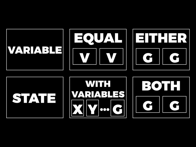
Surprisingly, these six pieces are enough to make a simple relational language called μKanren. It was presented in a paper published only two years ago, in 2013, by Jason Hemann and Daniel Friedman.
μKanren is part of the miniKanren family of languages. The full miniKanren language has more complex primitives that can be built out of the μKanren ones I’ve shown you.
What can it do?
So far we haven’t seen any convincing examples of our little language doing anything good — we’ve just been making variables equal to things, which is a bit underwhelming. To do something actually useful we need the goals to be able to work with data structures instead of just opaque values.
Fortunately, instead of trying to support every possible data structure, we can just support one: pairs. If a user of this language wants to use a more sophisticated data structure, they can build it out of pairs.
Pairs
Here’s how a pair should work:
>>pair = Pair.new(5, 9)=> (5, 9) >>pair.left=> 5 >>pair.right=> 9
We should be able to make a pair of two values, and then later retrieve the left or the right value from the pair.
Fortunately Ruby makes that very easy for us to implement. We can just use a Struct:
Pair = Struct.new(:left, :right) do
  def inspect
    "(#{left.inspect}, #{right.inspect})"
  end
end
The implementation of #inspect lets us see nicely-formatted values in IRB.
Getting our language to “support pairs” means teaching unification to look inside them. For example:
>> goal = Goal.with_variables { |x, y|
     Goal.equal(
       Pair.new(3, x),
       Pair.new(y, Pair.new(5, y))
     )
   }
=> #<Goal @block=#<Proc>>
This goal is trying to make a pair of 3 and x equal to a pair of y and a nested pair of 5 and y. It might not be obvious how to make those things equal, but our unification procedure needs to be able to do it:
>>states = goal.pursue_in(State.new)=> #<Enumerator: #<Enumerator::Generator>:each> >>state = states.first=> #<State @variables=[x, y], @values={y=>3, x=>(5, 3)}> >>state.values=> {y=>3, x=>(5, 3)}
The answer is that y has to be 3 and x has to be the pair (5, 3). This can only work if unification knows how to look inside a pair and make it equal to another pair.
That’s actually pretty easy to do. We can take our existing definition of #unify and add an extra clause to it:
class State
  def unify(a, b)
    a, b = value_of(a), value_of(b)

    if a == b
      self
    elsif a.is_a?(Variable)
      assign_values a => b
    elsif b.is_a?(Variable)
      assign_values b => a
    elsif a.is_a?(Pair) && b.is_a?(Pair)
      state = unify(a.left, b.left)
      state.unify(a.right, b.right) if state
    end
  end
end
If #unify finds that it’s trying to make two pairs equal, it just unifies the left elements of the pairs and then unifies the right elements in the resulting state.
We need to teach #value_of to go inside pairs as well: if we ask it for the value of a pair like (x, y), it should be able to extract x and y from the pair, find both their values, and return the pair of them as a result.
It’s easy enough to do that by adding a clause to #value_of:
class State
  def value_of(key)
    if values.has_key?(key)
      value_of values.fetch(key)
    elsif key.is_a?(Pair)
      Pair.new(
        value_of(key.left),
        value_of(key.right)
      )
    else
      key
    end
  end
end
Another little convenience is that the state already keeps track of all the variables that have been declared within it, so instead of looking up variables explicitly by asking “what’s the value of the variable called x?”, we can just ask the state to give us the values of its first few variables:
class State
  def results(n)
    variables.first(n).
      map { |variable| value_of(variable) }
  end

  def result
    results(1).first
  end
end
The #results method finds the first n variables in the state and returns their values, and the shorthand #result method just returns the value of the state’s first variable.
That’s nice because now, whenever we have a state, we can just ask “what’s the value of your first two variables?”, without needing to handle the variables ourselves:
>>state.values=> {y=>3, x=>(5, 3)} >>state.variables=> [x, y] >>state.results 2=> [(5, 3), 3]
And it’s even nicer to just be able to ask, “what’s your result?”:
>> state.result
=> (5, 3)
This is just a little convention — when we receive a state containing lots of variables, we can ask it for its result and get the value of its first variable.
Pairs are a little bit boring, but now that we’ve supported them in #unify and #value_of we can build other data structures out of them, and then things start to get interesting.
Lists
For example, as you may know, we can use pairs to encode an array by using a representation called a list.
If we want to represent an array of three values, we can do that by making three nested pairs containing those values along with a magic value that means “empty list”.
![The array ['a', 'b', 'c'] becomes the pairs ('a', ('b', ('c', ∙)))](images/hello-declarative-world/list.png)
Here’s how we could do that in Ruby:
EMPTY_LIST = :empty

def to_list(array)
  if array.empty?
    EMPTY_LIST
  else
    first, *rest = array
    Pair.new(first, to_list(rest))
  end
end
First we pick some special value to represent the empty list — we’re just using the symbol :empty here — and then we write a helper method to recursively convert an array into a list by building nested pairs. If the array is empty then the helper method returns the special empty list value, otherwise it extracts the first element of the array and pairs it up with the result of turning the rest of the array into a list.
If we call #to_list with an array of strings, we get back a list made from nested pairs:
>> to_list ['a', 'b', 'c']
=> ('a', ('b', ('c', :empty)))
We’d like to be able to convert a list back into an array as well. Here’s how to do that:
def from_list(list)
  if list == EMPTY_LIST
    []
  else
    first, rest = list.left, list.right
    [first, *from_list(rest)]
  end
end
If #from_list is called with the empty list then it returns an empty array, otherwise it recursively converts the tail of the list to an array and prepends the head of the list.
So we can turn a list back into an array too:
>> from_list \
     Pair.new('a',
       Pair.new('b',
         Pair.new('c', EMPTY_LIST)
       )
     )
=> ['a', 'b', 'c']
Now that we can turn Ruby’s native arrays into lists, and turn those back into arrays again, we have a way of talking about arrays in our goals. That means we have the power to write goals that make arrays equal. For example:
>> goal = Goal.with_variables { |x, y, z|
     Goal.equal(
       to_list([x, 2, z]),
       to_list([1, y, 3])
     )
   }
=> #<Goal @block=#<Proc>>
This goal tries to make the array [x, 2, z] equal to the array [1, y, 3]. Here’s what happens when we pursue it:
>>states = goal.pursue_in(State.new)=> #<Enumerator: #<Enumerator::Generator>:each> >>states.next.values=> {x=>1, y=>2, z=>3}
Pursuing the goal produces a state where x is equal to 1, y is equal to 2 and z is equal to 3. So the goal has been able to compare the two arrays and match up their elements even though we haven’t built explicit support for arrays into the language, because the arrays have been encoded using pairs.
This is particularly interesting because we can also use goals to define operations on the structure of lists, not just individual opaque values inside them.
Here’s a method called #append:
def append(a, b, c)
  Goal.either(
    Goal.both(
      Goal.equal(a, EMPTY_LIST),
      Goal.equal(b, c)
    ),
    Goal.with_variables { |first, rest_of_a, rest_of_c|
      Goal.both(
        Goal.both(
          Goal.equal(a, Pair.new(first, rest_of_a)),
          Goal.equal(c, Pair.new(first, rest_of_c))
        ),
        append(rest_of_a, b, rest_of_c)
      )
    }
  )
end
#append builds a goal which says: the lists a and b joined together are equal to the list c. It’s not worth dwelling on the implementation details, but notice that it’s just built out of our four basic goals. Briefly, it works by saying:
- either
ais equal to the empty list, in which casebandcare the same, because appending something to the empty list doesn’t change it; - or
aandcboth have the same first element, and if you append the rest ofa’s elements withb, you get the rest ofc. (There’s a recursive call at the bottom, which talks about appending some smaller lists.)
Don’t get too hung up on the details, but the important thing is that this is essentially a declarative definition of what it means for two lists to be appended to make a third one. It’s written it in a verbose way to make it easier to read, but it’s conceptually very simple.
What’s really interesting about this definition is that there’s no real “input” or “output” — it just constrains a, b and c to have a particular relationship. This definition is really more “relational” than it is “functional”: it defines a specific relation called “append”, and any given values of a, b and c may or may not be related in this specific way.
We can use goals to query this append relation. For example, we can make a goal which says that ['h', 'e'] appended with ['l', 'l', 'o'] is equal to the variable x:
>> goal = Goal.with_variables { |x|
     append(
       to_list(['h', 'e']),
       to_list(['l', 'l', 'o']),
       x
     )
   }
=> #<Goal @block=#<Proc>>
If we pursue that goal in an empty state…
>>states = goal.pursue_in(State.new)=> #<Enumerator: #<Enumerator::Generator>:each> >>state.next.result=> ("h", ("e", ("l", ("l", ("o", :empty))))) >>from_list _=> ["h", "e", "l", "l", "o"]
…we find that the value of x that satisfies this relation is the list encoding of the array ['h', 'e', 'l', 'l', 'o'].
But because our append goal expresses a relation between values instead of a one-way function, we can put that variable in other places. We can ask: if I append x and ['l', 'o'], and the result is ['h', 'e', 'l', 'l', 'o'], what is x?
>>goal = Goal.with_variables { |x| append( x, to_list(['l', 'o']), to_list(['h', 'e', 'l', 'l', 'o']) ) }=> #<Goal @block=#<Proc>> >>states = goal.pursue_in(State.new)=> #<Enumerator: #<Enumerator::Generator>:each> >>from_list states.next.result=> ["h", "e", "l"]
The answer is that x is ['h', 'e', 'l']. This is like running a conventional append function backwards, and we get that for free. That’s pretty surprising!
Here’s something even more surprising. We can ask: if appending x and y produces ['h', 'e', 'l', 'l', 'o'], then what are x and y?
>>goal = Goal.with_variables { |x, y| append( x, y, to_list(['h', 'e', 'l', 'l', 'o']) ) }=> #<Goal @block=#<Proc>> >>states = goal.pursue_in(State.new)=> #<Enumerator: #<Enumerator::Generator>:each> >>states.next.results(2)=> [:empty, ("h", ("e", ("l", ("l", ("o", :empty)))))] >>_.map { |list| from_list(list) }=> [[], ["h", "e", "l", "l", "o"]]
The result state says that x is [] and y is ['h', 'e', 'l', 'l', 'o'], so it’s found values of x and y that satisfy the constraint.
But there are more states in the stream! Let’s get the next one:
>> states.next.results(2).map { |list| from_list(list) }
=> [["h"], ["e", "l", "l", "o"]]
It says that x is ['h'], and y is ['e', 'l', 'l', 'o'].
The next state says x is ['h', 'e'] and y is ['l', 'l', 'o']:
>> states.next.results(2).map { |list| from_list(list) }
=> [["h", "e"], ["l", "l", "o"]]
In fact, if we just start the stream again and iterate over it, we get all possible combinations of values that make ['h', 'e', 'l', 'l', 'o'] when appended together:
>>states = goal.pursue_in(State.new)=> #<Enumerator: #<Enumerator::Generator>:each> >>states.each do |state| p state.results(2).map { |list| from_list(list) } end[[], ["h", "e", "l", "l", "o"]] [["h"], ["e", "l", "l", "o"]] [["h", "e"], ["l", "l", "o"]] [["h", "e", "l"], ["l", "o"]] [["h", "e", "l", "l"], ["o"]] [["h", "e", "l", "l", "o"], []] => nil
So not only can we run functions backwards, we can also discover multiple “inputs” that produce the desired “output”. It’s pretty interesting that we can get that behaviour just by expressing what it means to append two lists, and also interesting that this functionality emerges from the simple primitives we built.
Under the hood this is happening through a fairly mundane search strategy encoded in the primitives we built, but the useful thing is the way we’ve expressed the computation we’re interested in and the flexibility of how we’ve been able to interact with it.
Numbers
Let’s briefly try another trick. Instead of encoding arrays as pairs, let’s try encoding numbers. There’s a simple encoding called Peano numbers, where we represent the number 3 as three nested pairs each containing a special increment marker, along with some special zero marker value at the end. It looks like a list of three dummy values:
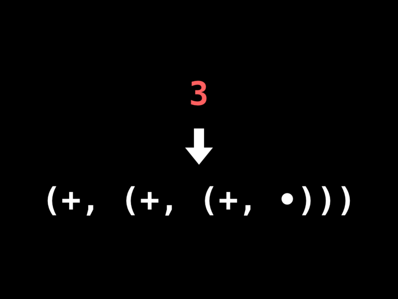
Here’s how we translate numbers into that encoding. We choose special values to represent zero and increment, and define a method that recursively converts a number into nested pairs:
ZERO, INC = :z, :+

def to_peano(number)
  if number.zero?
    ZERO
  else
    Pair.new(INC, to_peano(number - 1))
  end
end
If we pass in the number 3, it gets turned into three nested pairs:
>> to_peano 3
=> (:+, (:+, (:+, :z)))
We can go the other way too, by starting from zero and recursively incrementing it the appropriate number of times:
def from_peano(peano)
  if peano == ZERO
    0
  else
    from_peano(peano.right) + 1
  end
end
So we can turn three nested pairs back into the Ruby number 3:
>> from_peano \
     Pair.new(INC,
       Pair.new(INC,
         Pair.new(INC, ZERO)
       )
     )
=> 3
Again, this ability to turn numbers into pairs and back again means that we can start talking about them in goals.
For example, we can define a goal like add:
def add(x, y, z)
  Goal.either(
    Goal.both(
      Goal.equal(x, ZERO),
      Goal.equal(y, z)
    ),
    Goal.with_variables { |smaller_x, smaller_z|
      Goal.both(
        Goal.both(
          Goal.equal(x, Pair.new(INC, smaller_x)),
          Goal.equal(z, Pair.new(INC, smaller_z))
        ),
        add(smaller_x, y, smaller_z)
      )
    }
  )
end
This goal says that x added to y is equal to z. It’s similar to append: either x is zero, in which case y and z are the same, or x and z aren’t zero, in which case you can add y to the number one less than x to get the number one less than z. This declaratively specifies what it means for two numbers to add up to a third number.
Once we have #add, we can ask: if 5 added to 3 is x, then what is the value of x?
>> goal = Goal.with_variables { |x|
     add(
       to_peano(5),
       to_peano(3),
       x
     )
   }
=> #<Goal @block=#<Proc>>
When we pursue that goal, we get the answer 8:
>>states = goal.pursue_in(State.new)=> #<Enumerator: #<Enumerator::Generator>:each> >>states.next.result=> (:+, (:+, (:+, (:+, (:+, (:+, (:+, (:+, :z)))))))) >>from_peano _=> 8
But as with append, we can also ask a different kind of question, like: what x added to 3 is equal to 8?
>>goal = Goal.with_variables { |x| add( x, to_peano(3), to_peano(8) ) }=> #<Goal @block=#<Proc>> >>states = goal.pursue_in(State.new)=> #<Enumerator: #<Enumerator::Generator>:each> >>from_peano states.next.result=> 5
We get the answer 5. So by defining the notion of addition, we get subtraction for free, just by following the same relation in a different direction.
And we can ask: if x added to y is 8, what are x and y?
>>goal = Goal.with_variables { |x, y| add(x, y, to_peano(8)) }=> #<Goal @block=#<Proc>> >>states = goal.pursue_in(State.new)=> #<Enumerator: #<Enumerator::Generator>:each> >>states.each do |state| p state.results(2).map { |peano| from_peano(peano) } end[0, 8] [1, 7] [2, 6] [3, 5] [4, 4] [5, 3] [6, 2] [7, 1] [8, 0] => nil
We find that x and y can be 0 and 8, or 1 and 7, or 2 and 6, and so on.
One last thing! Here’s another relation on numbers: x multiplied by y equals z.
def multiply(x, y, z)
  Goal.either(
    Goal.both(
      Goal.equal(x, ZERO),
      Goal.equal(z, ZERO)
    ),
    Goal.with_variables { |smaller_x, smaller_z|
      Goal.both(
        Goal.both(
          Goal.equal(x, Pair.new(INC, smaller_x)),
          add(smaller_z, y, z)
        ),
        multiply(smaller_x, y, smaller_z)
      )
    }
  )
end
It’s a similar deal: either x and z are both zero, because zero multiplied by anything is zero, or they’re not zero, and knocking y off z produces the same number as knocking one off x and multiplying by y. That’s confusing but it’s true; it just describes what multiplication is.
But the point of this is that we can ask: what’s 3 multiplied by 8?
>> goal = Goal.with_variables { |x|
     multiply(
       to_peano(3),
       to_peano(8),
       x
     )
   }
=> #<Goal @block=#<Proc>>

>> states = goal.pursue_in(State.new)
=> #<Enumerator: #<Enumerator::Generator>:each>

>> states.next.result
=> (:+, (:+, (:+, (:+, (:+, (:+, (:+, (:+,
   (:+, (:+, (:+, (:+, (:+, (:+, (:+, (:+,
   (:+, (:+, (:+, (:+, (:+, (:+, (:+, (:+,
   :z))))))))))))))))))))))))

>> from_peano _
=> 24
The answer is twenty-four.
To finish, let’s ask what x and y can be if their product is 24:
>>goal = Goal.with_variables { |x, y| multiply( x, y, to_peano(24) ) }=> #<Goal @block=#<Proc>> >>states = goal.pursue_in(State.new)=> #<Enumerator: #<Enumerator::Generator>:each> >>states.take(8).each do |state| p state.results(2).map { |peano| from_peano(peano) } end[1, 24] [2, 12] [3, 8] [4, 6] [6, 4] [8, 3] [12, 2] [24, 1] => nil
Our system is powerful enough to factorise 24 and tell us that x and y can be 1 and 24, or 2 and 12, or 3 and 8, and so on.
Of course, this is just an illustration of what’s possible. We can make other more complex data structures than lists and Peano numbers, and ask more complex questions about them.
Conclusion
That was a bit of a whirlwind, but hopefully it’s given you a glimpse of what’s possible with declarative programming.
In your journey as a programmer I would encourage you to think beyond the low-level details of how computing machines work, and consider alternative models of programming. Think about how programming can be a collaboration between you and the computer, not you just barking instructions at it.
Instead of giving computers imperative recipes for doing things, you can give them declarative specifications of problems and let them find the answers. As a human your skill is understanding what needs to be done; the computer’s skill is working out the best way to do it.
If you only ever do imperative work, you can end up wasting your time and the computer’s time. Some people have to spend some of their time doing this boring imperative stuff with computers, but there’s no reason why we all have to do that all of the time.
Instead we can design these systems where we first build a reliable core of imperative instructions that knows how to solve declarative problems, and then spend our day-to-day programming time thinking about describing those problems correctly, ignoring the “playing computer” detail of a linear sequence of instructions going through a CPU.
Right now this is only an aspiration, not the actual world we live in! But things are changing; React is bringing the idea of declarative programming to a much wider audience, as are technologies like the Cassowary constraint solver which drives the Auto Layout system for iOS and OS X by solving linear constraints to dynamically arrange a user interface.
All of those things do give me a little bit of hope. In spite of the fact that John Backus’s rant didn’t really change the world in the way he wanted it to, I do think that things are changing, so maybe one day we really could live in that declarative world.
