The computational behaviour of Ruby procs (aka “lambdas” and “anonymous functions”) gives us enough power to implement any data structure and algorithm. Let’s reimplement that behaviour from scratch and then explore how to make our implementation more efficient.
This is a lightly edited transcript of a talk I gave at RubyConf 2021, for which the video, slides and code are available. Some of the ideas are also covered in my O’Reilly book.
Almost exactly ten years ago, right at the end of October 2011, I gave a talk called Programming with Nothing at the Ruby Manor conference in London.
The details of that talk aren’t important — you can watch it or read a transcript if you’re interested in understanding it — but I’ll summarise its conclusion so that I can build on it.
In that talk I showed that we can still write useful programs in Ruby if we only allow ourselves to create procs and call procs. And that’s because — it turns out! — we can use procs to encode any data structure, and then use procs to implement operations on those encoded data structures.
Here’s one way to encode a number as a proc that you call once with a function p, then again with an argument x, and it calls p on x a fixed number of times:
ZERO  = -> p { -> x {       x    } }
ONE   = -> p { -> x {     p[x]   } }
TWO   = -> p { -> x {   p[p[x]]  } }
THREE = -> p { -> x { p[p[p[x]]] } }
For example, the encoding of the number three calls p three times. Not surprisingly, this encoding lets us represent numbers that are as large as we like:
FIVE    = -> p { -> x { p[p[p[p[p[x]]]]] } }
FIFTEEN = -> p { -> x { p[p[p[p[p[p[p[p[p[p[p[p[p[p[p[x]]]]]]]]]]]]]]] } }
HUNDRED = -> p { -> x { p[p[p[p[p[p[p[p[p[p[p[p[p[p[p[p[p[p[p[p[p[p[p[p[p[
p[p[p[p[p[p[p[p[p[p[p[p[p[p[p[p[p[p[p[p[p[p[p[p[p[p[p[p[p[p[p[p[p[p[p[p[p[
p[p[p[p[p[p[p[p[p[p[p[p[p[p[p[p[p[p[p[p[p[p[p[p[p[p[p[p[p[p[p[p[p[p[p[p[p[
p[x]]]]]]]]]]]]]]]]]]]]]]]]]]]]]]]]]]]]]]]]]]]]]]]]]]]]]]]]]]]]]]]]]]]]]]]
]]]]]]]]]]]]]]]]]]]]]]]]]]]]] } }
These encodings are legitimate because there’s a way to convert them back into Ruby Integer objects whenever we like. If we take the Ruby proc that adds one to its argument, and call it on the Ruby 0 object three times, we get the Ruby 3 object:
>> THREE[-> n { n + 1 }][0]
=> 3
And the same thing works for a hundred:
>> HUNDRED[-> n { n + 1 }][0]
=> 100
If we call the proc zero times then we just get the original Ruby 0 object back:
>> ZERO[-> n { n + 1 }][0]
=> 0
Proc-encoded numbers are usable for computation because we can implement operations like increment, decrement, add and subtract in the same way:
INCREMENT = -> n { -> p { -> x { p[n[p][x]] } } }
DECREMENT = -> n { -> f { -> x { n[-> g { -> h { h[g[f]] } }] \
                                  [-> y { x }][-> y { y }] } } }

ADD      = -> m { -> n { n[INCREMENT][m] } }
SUBTRACT = -> m { -> n { n[DECREMENT][m] } }
MULTIPLY = -> m { -> n { n[ADD[m]][ZERO] } }
POWER    = -> m { -> n { n[MULTIPLY[m]][ONE] } }
These are a little complex so I won’t go into the details, but what’s relevant here is that they work. We can add an encoded five and three together to get an encoded eight, and then convert it back to an Integer to confirm its correctness:
>> EIGHT = ADD[FIVE][THREE]
=> #<Proc (lambda)>

>> EIGHT[-> n { n + 1 }][0]
=> 8
Similarly we can raise an encoded two to the power of an encoded eight, and when we decode it we get the Ruby number 256 as expected:
>> POWER[TWO][EIGHT][-> n { n + 1 }][0]
=> 256
We can encode more complex data structures like pairs and lists, including operations like checking for the empty list or fetching the first list item or the rest of the items…
PAIR  = -> x { -> y { -> f { f[x][y] } } }
LEFT  = -> p { p[-> x { -> y { x } }] }
RIGHT = -> p { p[-> x { -> y { y } }] }

EMPTY    = PAIR[TRUE][TRUE]
UNSHIFT  = -> l { -> x {
             PAIR[FALSE][PAIR[x][l]]
           } }
IS_EMPTY = LEFT
FIRST    = -> l { LEFT[RIGHT[l]] }
REST     = -> l { RIGHT[RIGHT[l]] }
…and more complex operations like generating an encoded list of all encoded numbers within a certain range of values, or mapping an arbitrary function over an encoded list:
RANGE =
  Z[-> f {
    -> m { -> n {
      IF[IS_LESS_OR_EQUAL[m][n]][
        -> x {
          UNSHIFT[f[INCREMENT[m]][n]][m][x]
        }
      ][
        EMPTY
      ]
    } }
  }]

MAP =
  -> k { -> f {
    FOLD[k][EMPTY][
      -> l { -> x { UNSHIFT[l][f[x]] } }
    ]
  } }
That gives us everything we need to entirely implement FizzBuzz with all its data and operations encoded as procs.
FIZZBUZZ =
  MAP[RANGE[ONE][HUNDRED]][-> n {
    IF[IS_ZERO[MOD[n][FIFTEEN]]][
      FIZZ_BUZZ
    ][IF[IS_ZERO[MOD[n][THREE]]][
      FIZZ
    ][IF[IS_ZERO[MOD[n][FIVE]]][
      BUZZ
    ][
      TO_DIGITS[n]
    ]]]
  }]
At the end of the Programming with Nothing talk I show that we can expand all the constants to get a complete FizzBuzz implementation which is syntactically just procs. We can check it works by pasting it into a terminal and using some helper methods to decode it into an array of strings:
>> FIZZBUZZ = -> k { -> f { -> f { -> x { f[-> y { x[x][y] }] }[-> x { f[-> y { …
=> #<Proc (lambda)>

>> to_array(FIZZBUZZ).each do |s| puts to_string(s) end
1
2
Fizz
4
Buzz
Fizz
7
8
Fizz
Buzz
⋮
It slows down a bit towards the end as the numbers get larger. On my laptop it takes about 18 seconds to print all hundred strings.
It’s ten years later and I’d like to pull on this thread a little more. Programming with Nothing showed that an extremely minimal subset of Ruby is still a fully capable programming language, so we’re getting essentially all the computational power of Ruby while only relying on a tiny fraction of its features. Now I’d like us to better understand that fraction by actually implementing it ourselves from scratch. That means asking three questions:
Could we represent these encoded values ourselves? In other words: instead of using procs to represent numbers and lists and stuff, could we design and implement our own objects to do it?
If we have our own objects for encoding values, can we explicitly evaluate them and recreate the computational behaviour that we get for free with procs?
If we do manage to recreate that behaviour and perform computations with our objects, can we decode the results back into useful information afterwards?
If we could do all three of these things, we’d no longer be relying on Ruby’s built-in implementation of procs to bring our encodings to life; we’d have constructed our own implementation that we can understand and control, and I think that would be pretty cool.
Let’s start with that first question: could we represent these encoded values ourselves? Can we roll our sleeves up and construct our own honest hard-working artisanal data structure to represent encoded values, instead of lounging around expecting Ruby to be cool with us taking as many procs as we like and using them to represent whatever we want to?
Yeah, I think we can. Consider some arbitrary Ruby value encoded as procs:
-> p { -> x { p[p[p[x]]] } }This was our encoding of the number three. Appropriately enough, there are only three kinds of syntax appearing here:
There are some variables. There are four of them here: three variables named p, and one variable named x.
There are three calls: the inner p[x], the middle p[p[x]] and the outer p[p[p[x]]].
There are two proc definitions, each with a parameter name and a body: there’s the outer one -> p { … } with the parameter name p, whose body is another proc definition; and the inner one -> x { … } with the parameter name x, whose body is the outermost of those three nested calls.
The simplicity of this setup is good news. If we want to represent an expression like this, we’ll only need to worry about representing variables, calls and definitions, because those are the only three structural features that we see in any of these encoded values, even a really big one like FIZZBUZZ. We can think of any proc-encoded expression as a wiring diagram which connects parameters to variables in an intricate and very specific way to achieve its computational behaviour.
We can use Ruby’s Struct class to make our own representation of expressions. We need classes for variables, calls and definitions, each with the relevant members:
Variable = Struct.new(:name)

Call = Struct.new(:receiver, :argument)

Definition = Struct.new(:parameter, :body)
A variable has a name, a call has a receiver and an argument — the receiver is the thing being called, and the argument is the value being passed to it — and a proc definition has a parameter name and a body.
To make these structs easier to work with, we can implement the #inspect method on each class so their instances get formatted nicely when we look at them in IRB:
Variable = Struct.new(:name) do
  def inspect = "#{name}"
end

Call = Struct.new(:receiver, :argument) do
  def inspect = "#{receiver.inspect}[#{argument.inspect}]"
end

Definition = Struct.new(:parameter, :body) do
  def inspect = "-> #{parameter} { #{body.inspect} }"
end
Now we can make a new variable whose name is x, or a new call whose receiver and argument are that variable x, or a new definition whose body is that call:
>> variable = Variable.new(:x)
=> x

>> call = Call.new(variable, variable)
=> x[x]

>> definition = Definition.new(:x, call)
=> -> x { x[x] }
They look superficially like the real thing because those #inspect methods format them to look like Ruby source code. But they’re not real variables or procs, they’re structures made out of objects whose behaviour we control.
As another example, we can make a big inline structure like this to represent the encoding of the number three:
>> three =
     Definition.new(:p,
       Definition.new(:x,
         Call.new(
           Variable.new(:p),
           Call.new(
             Variable.new(:p),
             Call.new(
               Variable.new(:p),
               Variable.new(:x)
             )
           )
         )
       )
     )
=> -> p { -> x { p[p[p[x]]] } }
If we look at the shape of this three object, it’s really a tree structure:
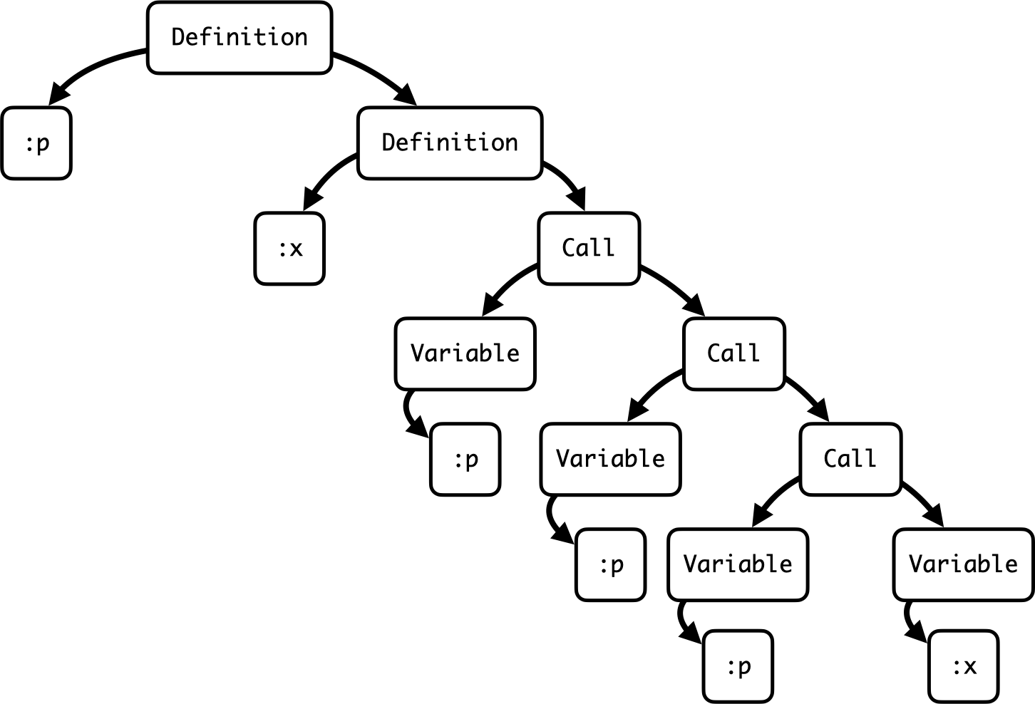
Inside the top-level definition there’s a parameter name :p and another definition. Within that definition there’s another parameter name :x and a call, and inside that call there are some nested calls and variables.
We usually call this kind of structure an abstract syntax tree, so this is the abstract syntax tree of the proc encoding of the number three.
We’ve seen that representing these encoded values as trees is not difficult. But if we already have an encoded value as a Ruby proc object in memory, like the number THREE or FIZZBUZZ or whatever, how can we convert it into our abstract syntax tree representation?
I can think of a couple of hacky ways of doing that. The first way is to ask MRI for the YARV bytecode instructions which we could presumably walk over and figure out the structure of the proc, or use the #disassemble method to generate the human-readable version and process that somehow:
>> instructions = RubyVM::InstructionSequence.of(-> p { -> x { p[p[p[x]]] } })
=> <RubyVM::InstructionSequence:block in <main>@(irb):1>

>> instructions.to_a
=> ["YARVInstructionSequence/SimpleDataFormat", 3, 0, 1, {:arg_size=>1,
   :local_size=>1, :stack_max=>1, :node_id=>19, :code_location=>[1, 49, 1, 74]},
   "block in <main>", "(irb)", "(irb)", 1, :block, [:p], {:lead_num=>1,
   :ambiguous_param0=>true}, [[:redo, nil, :label_1, :label_6, :label_1, 0],
   [:next, nil, :label_1, :label_6, :label_6, 0]], [1, :RUBY_EVENT_B_CALL, [:nop],
   :label_1, :RUBY_EVENT_LINE, [:putspecialobject, 1], [:send, {:mid=>:lambda,
   :flag=>4, :orig_argc=>0}, ["YARVInstructionSequence/SimpleDataFormat", 3, 0, 1,
   {:arg_size=>1, :local_size=>1, :stack_max=>4, :node_id=>17, :code_location=>[1,
   56, 1, 72]}, "block (2 levels) in <main>", "(irb)", "(irb)", 1, :block,
   [:x], {:lead_num=>1, :ambiguous_param0=>true}, [[:redo, nil, :label_1,
   :label_15, :label_1, 0], [:next, nil, :label_1, :label_15, :label_15, 0]], [1,
   :RUBY_EVENT_B_CALL, [:nop], :label_1, :RUBY_EVENT_LINE, [:getlocal_WC_1, 3],
   [:getlocal_WC_1, 3], [:getlocal_WC_1, 3], [:getlocal_WC_0, 3], [:opt_aref,
   {:mid=>:[], :flag=>16, :orig_argc=>1}], [:opt_aref, {:mid=>:[], :flag=>16,
   :orig_argc=>1}], [:opt_aref, {:mid=>:[], :flag=>16, :orig_argc=>1}], :label_15,
   [:nop], :RUBY_EVENT_B_RETURN, [:leave]]]], :label_6, [:nop],
   :RUBY_EVENT_B_RETURN, [:leave]]]

>> puts instructions.disassemble
== disasm: #<ISeq:block in <main>@(irb):1 (1,49)-(1,74)> (catch: FALSE)
== catch table
| catch type: redo   st: 0001 ed: 0006 sp: 0000 cont: 0001
| catch type: next   st: 0001 ed: 0006 sp: 0000 cont: 0006
|------------------------------------------------------------------------
local table (size: 1, argc: 1 [opts: 0, rest: -1, post: 0, block: -1, kw: -1@-1, kwrest: -1])
[ 1] p@0<Arg>
0000 nop                                                              (   1)[Bc]
0001 putspecialobject                       1[Li]
0003 send                                   <calldata!mid:lambda, argc:0, FCALL>, block (2 levels) in <main>
0006 nop
0007 leave                                                            (   1)[Br]

== disasm: #<ISeq:block (2 levels) in <main>@(irb):1 (1,56)-(1,72)> (catch: FALSE)
== catch table
| catch type: redo   st: 0001 ed: 0015 sp: 0000 cont: 0001
| catch type: next   st: 0001 ed: 0015 sp: 0000 cont: 0015
|------------------------------------------------------------------------
local table (size: 1, argc: 1 [opts: 0, rest: -1, post: 0, block: -1, kw: -1@-1, kwrest: -1])
[ 1] x@0<Arg>
0000 nop                                                              (   1)[Bc]
0001 getlocal_WC_1                          p@0[Li]
0003 getlocal_WC_1                          p@0
0005 getlocal_WC_1                          p@0
0007 getlocal_WC_0                          x@0
0009 opt_aref                               <calldata!mid:[], argc:1, ARGS_SIMPLE>
0011 opt_aref                               <calldata!mid:[], argc:1, ARGS_SIMPLE>
0013 opt_aref                               <calldata!mid:[], argc:1, ARGS_SIMPLE>
0015 nop
0016 leave                                                            (   1)[Br]
The second way is that, if we know the proc was loaded from a file, we could use #source_location to find out which line in which file, read it in as a string, and use Ripper from the standard library to parse that string into a structure that we can examine:
$ echo 'THREE = -> p { -> x { p[p[p[x]]] } }' > three.rb

$ irb -I.
>> require 'three'
=> true

>> file_name, line_number = THREE.source_location
=> ["three.rb", 1]

>> line = IO.readlines(file_name)[line_number - 1]
=> "THREE = -> p { -> x { p[p[p[x]]] } }\n"

>> pp Ripper.sexp(line)
[:program,
 [[:assign,
   [:var_field, [:@const, "THREE", [1, 0]]],
   [:lambda,
    [:params, [[:@ident, "p", [1, 11]]], nil, nil, nil, nil, nil, nil],
    [[:lambda,
      [:params, [[:@ident, "x", [1, 18]]], nil, nil, nil, nil, nil, nil],
      [[:aref,
        [:var_ref, [:@ident, "p", [1, 22]]],
        [:args_add_block,
         [[:aref,
           [:var_ref, [:@ident, "p", [1, 24]]],
           [:args_add_block,
            [[:aref,
              [:var_ref, [:@ident, "p", [1, 26]]],
              [:args_add_block,
               [[:var_ref, [:@ident, "x", [1, 28]]]],
               false]]],
            false]]],
         false]]]]]]]]]
I don’t think either of these options is very good. The first one only works on MRI, because YARV is MRI-specific; the second one only works if we have the source code of our proc available as a file, which in general we might not if it’s been constructed at runtime.
I’m going to suggest a third option: use the behaviour of a proc to reveal its inner structure. That would mean we’re only relying on the functionality of the proc itself and not making any assumptions about where it came from or whether implementation-specific Ruby internals are available.
We can already ask Ruby about the parameters of a proc like THREE:
>> THREE = -> p { -> x { p[p[p[x]]] } }
=> #<Proc (lambda)>

>> THREE.parameters
=> [[:req, :p]]

>> parameter = THREE.parameters[0][1]
=> :p
This is telling us that THREE has one required parameter whose name is :p, and it’s easy to pull out that name, which is half of what we want to know about the proc definition. But how do we get its body?
Let’s think about the easier case of a proc called IDENTITY which just returns its argument:
>> IDENTITY = -> x { x }
=> #<Proc (lambda)>

>> IDENTITY.parameters
=> [[:req, :x]]
All we know from the outside is that its parameter is called x. We can’t retrieve its body directly, but we do know that, when we call it, whatever argument we pass in is going to replace all of the occurrences of x in its body.
If we make a Variable instance called x that we want to represent the occurrences of the parameter, we can call the proc with that object and get back its body, which is just our Variable instance x again:
>> variable = Variable.new(IDENTITY.parameters[0][1])
=> x

>> body = IDENTITY.call(variable)
=> x
By doing this we’ve learned that the proc’s parameter is called x and its body is the variable x, which is correct. 🎉
Here’s another example, a proc called OMEGA which calls its argument with itself:
>> OMEGA = -> x { x[x] }
=> #<Proc (lambda)>
We can do the same trick and make a variable with the same name as its parameter, but when we try calling the proc with that variable we get an exception:
>> variable = Variable.new(OMEGA.parameters[0][1])
=> x

>> body = OMEGA.call(variable)
in `[]': no implicit conversion of Variable into Integer (TypeError)
This happens because the body is calling the #[] method on the variable we passed in, but since the variable is a Struct, that’s using the Struct#[] method which fetches the value of the member at a particular numeric index.
We can take advantage of this by redefining the #[] method on the Variable class so that, instead of calling or fetching anything, it builds a new Call instance which remembers the variable itself and the argument that was passed in:
>> class Variable
     def [](argument)
       Call.new(self, argument)
     end
   end
=> :[]
Now if we call the proc again, we get back a representation of its body:
>> body = OMEGA.call(variable)
=> x[x]
Nice! 👍🏻
Finally, let’s try with the proc encoding of the number three. We can make a variable p and call the proc with that variable as its argument. We get another proc back, because that’s what the body of THREE is:
>> THREE = -> p { -> x { p[p[p[x]]] } }
=> #<Proc (lambda)>

>> variable = Variable.new(THREE.parameters[0][1])
=> p

>> body = THREE.call(variable)
=> #<Proc (lambda)>
Fair enough, we can just repeat the procedure: make another variable from the inner proc’s parameter, named x this time, and call it with that variable. That gives us the body of the inner proc:
>> variable = Variable.new(body.parameters[0][1])
=> x

>> body.call(variable)
=> p[p[p[x]]]
Great. 🙌🏻 That tells us everything we need to completely reconstruct the original Ruby proc with our own representation.
We can wrap that technique up into a method which converts a proc into an abstract syntax tree:
def from_proc(proc)
  return proc unless proc.is_a?(Proc)

  case proc.parameters
  in [[:req, parameter]]
    argument = Variable.new(parameter)
    body = from_proc(proc.call(argument))
    Definition.new(parameter, body)
  end
end
This method uses the trick of creating a new Variable instance with the same name as the proc’s parameter and calling the proc with it as an argument, so that all occurrences of the proc’s parameter inside its body become that instance. Then we recursively convert the result, in case the proc’s body is another proc, and finish by building a new Definition instance.
As we just saw, to make this work we also need to replace the #[] method on the Variable, Call and Proc classes to convert the receiver and argument with #from_proc and wrap up the results in a new Call object:
[Variable, Call, Proc].each do |klass|
  klass.define_method :[] do |argument|
    receiver = from_proc(self)
    argument = from_proc(argument)
    Call.new(receiver, argument)
  end
end
I’ve picked those three classes because they’re the three kinds of object which can appear as the receiver of the #[] method inside a proc that we’re converting. So if we evaluate any proc body which contains a call, it’ll use this replacement method which builds an instance of our Call class instead of actually calling anything.
Now we can convert THREE into our own representation:
>> THREE
=> #<Proc (lambda)>
>> from_proc(THREE)
=> -> p { -> x { p[p[p[x]]] } }
>> from_proc(THREE).class
=> Definition
And likewise for FIZZBUZZ:
>> FIZZBUZZ
=> #<Proc (lambda)>
>> from_proc(FIZZBUZZ)
=> -> m { -> k { -> f { -> l { -> l { -> x { -> g { -> b { -> b { -> b { b }[b]
   }[b] }[-> p { -> p { -> p { p[-> x { -> y { x } }] }[p] }[p] }[l]][x][-> _ {
   g[-> _ { -> _ { -> _ { -> _ { -> x { -> x { -> x { -> x { -> f { -> f { -> f {
   -> f { -> l { -> x { -> g { -> b { -> b { -> b { -> b { -> b { b }[b] }[b] }[b]
   }[b] }[-> …
>> from_proc(FIZZBUZZ).class
=> Definition
Now that we have our own representation of these proc encodings, can we do the work of evaluating them ourselves so that we’re not relying on the behaviour of Ruby procs to compute two plus three, or FizzBuzz, or whatever?
That would mean implementing some method called #evaluate which can take an abstract syntax tree, called expression, and… you know… evaluate it somehow:
def evaluate(expression)
  case expression
  in Variable(name)
    # TODO — get value from the correct parameter?
  in Call(receiver, argument)
    # TODO — evaluate(receiver), evaluate(argument)?
  in Definition(parameter, body)
    # TODO — evaluate(body)?
  end
end
But it’s not very obvious what that means: a Variable will refer to the parameter of some proc that it’s inside, so maybe we can get an argument that way; and a Call will have a receiver and argument that need to be evaluated somehow and then we do something with them, I dunno what; and for a Definition we need to evaluate its body at some point, but not immediately, only later when it appears as part of a call somewhere else.
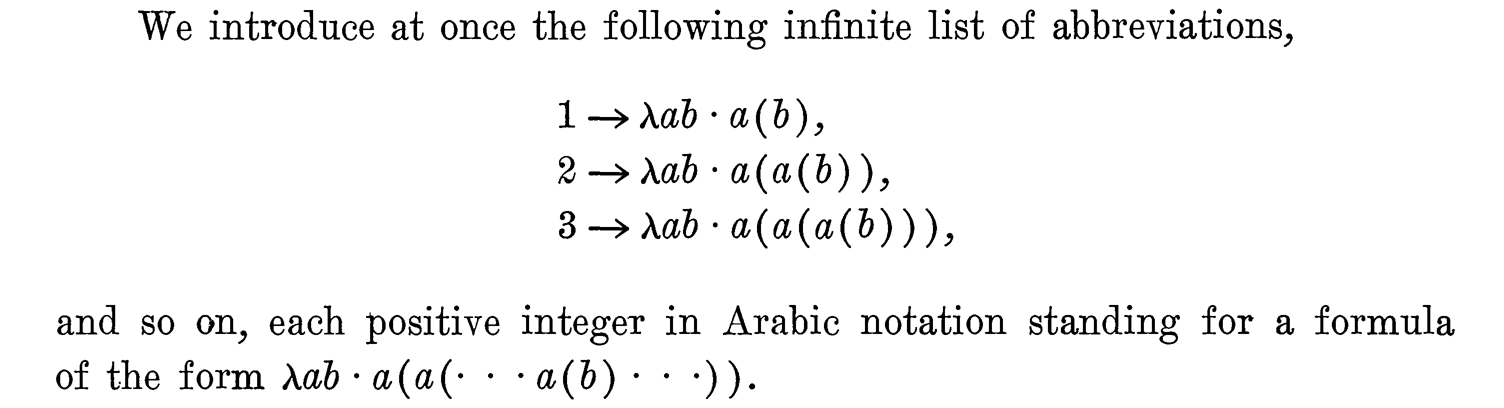
This is a bit complicated and I’m not clever enough to work it out myself. Fortunately, a mathematician called Alonzo Church wrote a paper in 1935 that explains how to do it.
It’s got tons of good stuff in it even though it’s over 85 years old. For example, there are some cool ideas about how to represent numbers as expressions which look like procs, which is ultimately the source of my entire previous talk, so… thanks Alonzo, I appreciate it:
But there’s also this bit about operations we can perform on these expressions:
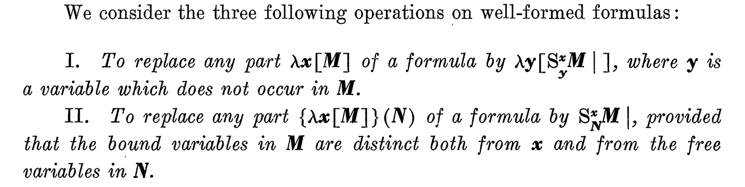
Operation number two here is called “reduction”, and in our Rubyist understanding, it’s talking about what to do when we call a proc with an argument. The notation is saying that the way to evaluate a call is to replace all occurrences of the variable named x in the expression M with the expression N. x is the name of the proc’s parameter, M is the body of the proc we’re calling, and N is the argument we’re calling it with. So, according to Church, replacing occurrences of variables inside proc bodies is pretty much all we need to implement.
Let’s briefly look at this reduction idea in the world of normal Ruby procs to see why it’s relevant. Say we have a proc p which takes a greeting and a name and returns an interpolated string:
>> p = -> greeting { -> name { "#{greeting}, #{name}!" } }
=> #<Proc (lambda)>
If we call p with the string 'Hello', we get another proc back:
>> p['Hello'] # -> name { "Hello, #{name}!" }
=> #<Proc (lambda)>
But conceptually what’s happened here is that the string 'Hello' has replaced the variable greeting in the body of p, so you can think of this result as being the body of p with one of its variables filled in with a value.
If we supply a second argument, the string 'RubyConf', we get back that inner string with both variables replaced with the two arguments we provided:
>> p['Hello']['RubyConf']
=> "Hello, RubyConf!"
In his 1935 paper, Church is saying that when we have a bunch of proc definitions and calls all stacked up together to make a big expression, we can get closer to a fully evaluated result by performing this reduction operation repeatedly. I’m going to quickly show you how we implement this operation on our abstract syntax tree representation.
First we need a helper method called #replace. It takes the name of the variable to replace, an expression to replace it with, and some original expression that we’re performing that replacement on:
def replace(name, replacement, original)
  case original
  in Variable(^name)
    replacement
  in Variable
    original
  in Call
    Call.new(
      replace(name, replacement, original.receiver),
      replace(name, replacement, original.argument)
    )
  in Definition(^name, _)
    original
  in Definition
    Definition.new(
      original.parameter,
      replace(name, replacement, original.body)
    )
  end
end
#replace recursively walks down the abstract syntax tree of the original expression. When it finds a variable whose name matches the one we’re looking for — by using the pinned ^name syntax in the first pattern, which will only match if the variable’s name is equal to the name we’re replacing — it’ll return the replacement expression instead of the original variable.
One interesting case is the Definition(^name, _) pattern, which matches a definition whose parameter name clashes with the name we’re replacing. At that point #replace stops recursing and returns the original definition, because any variables with that name inside the definition’s body must be references to its parameter, so we shouldn’t mess with them.
Here’s the #replace method in action. If we make three variables called a, b and c, and build an expression that calls a with b and c as arguments, we can use the #replace operation to replace b with some other expression, like the IDENTITY proc we saw earlier:
>> a, b, c = [:a, :b, :c].map { |name| Variable.new(name) }
=> [a, b, c]

>> expression = Call.new(Call.new(a, b), c)
=> a[b][c]

>> replace(:b, from_proc(-> x { x }), expression)
=> a[-> x { x }][c]
Or we could replace a or c instead, to get different expressions where a different variable has been replaced:
>> replace(:a, from_proc(-> x { x }), expression)
=> -> x { x }[b][c]

>> replace(:c, from_proc(-> x { x }), expression)
=> a[b][-> x { x }]
Once we have this #replace operation we can use it to reduce an expression by finding opportunities inside that expression to pull out the body of a definition and replace its variables with something else.
First we need another helper to decide whether an expression is a value — a successful result of evaluation:
def value?(expression)
  case expression
  in Definition
    true
  else
    false
  end
end
We’re using procs to encode values, so only proc definitions get to be a value; calls and variables aren‘t values.
Then we can finally implement that Alonzo Church reduction operation on expressions:
def reduce(expression)
  case expression
  in Call(receiver, argument) unless value?(receiver)
    Call.new(reduce(receiver), argument)
  in Call(receiver, argument) unless value?(argument)
    Call.new(receiver, reduce(argument))
  in Call(Definition(parameter, body), argument)
    replace(parameter, argument, body)
  end
end
Because Ruby uses a left-to-right call by value evaluation strategy, we have to do a bit of work to find the next part of the expression to reduce in the same order that Ruby would, so that we’re correctly reproducing its behaviour. In the general case we reduce the left-hand side of the call, which is the receiver; if the receiver is already a fully-reduced value then we reduce the right-hand side of the call instead, which is the argument; and then only in the special case when the receiver is definitely a definition, and the argument is a value, do we replace the parameter with the argument inside the receiver’s body, which is what Church said we should do.
To actually evaluate an expression, we just repeatedly reduce it. If we make expressions for add, one and two, then make an expression which calls add with one and two as arguments, we can keep reducing it over and over:
>> add, one, two = from_proc(ADD), from_proc(ONE), from_proc(TWO)
=> [-> m { -> n { n[-> n { -> p { -> x { p[n[p][x]] } } }][m] } }, -> p { -> x { p[x] } }, -> p { -> x { p[p[x]] } }]

>> expression = Call.new(Call.new(add, one), two)
=> -> m { -> n { n[-> n { -> p { -> x { p[n[p][x]] } } }][m] } }[-> p { -> x { p[x] } }][-> p { -> x { p[p[x]] } }]

>> expression = reduce(expression)
=> -> n { n[-> n { -> p { -> x { p[n[p][x]] } } }][-> p { -> x { p[x] } }] }[-> p { -> x { p[p[x]] } }]
>> expression = reduce(expression)
=> -> p { -> x { p[p[x]] } }[-> n { -> p { -> x { p[n[p][x]] } } }][-> p { -> x { p[x] } }]
>> expression = reduce(expression)
=> -> x { -> n { -> p { -> x { p[n[p][x]] } } }[-> n { -> p { -> x { p[n[p][x]] } } }[x]] }[-> p { -> x { p[x] } }]
>> expression = reduce(expression)
=> -> n { -> p { -> x { p[n[p][x]] } } }[-> n { -> p { -> x { p[n[p][x]] } } }[-> p { -> x { p[x] } }]]
>> expression = reduce(expression)
=> -> n { -> p { -> x { p[n[p][x]] } } }[-> p { -> x { p[-> p { -> x { p[x] } }[p][x]] } }]
>> expression = reduce(expression)
=> -> p { -> x { p[-> p { -> x { p[-> p { -> x { p[x] } }[p][x]] } }[p][x]] } }
>> expression = reduce(expression)
in `reduce': #<struct Definition> (NoMatchingPatternError)
If none of the patterns inside the #reduce method match, there’s no more reducing we can do, so evaluation is finished. We ended up with a definition at the top level, but Church only told us how to reduce calls – by doing some variable replacement on the body of the receiver — so it makes sense that we have to stop there.
That’s easy to wrap up as an #evaluate method. We just keep calling the #reduce method until none of the patterns inside it match:
def evaluate(expression)
  loop do
    expression = reduce(expression)
  rescue NoMatchingPatternError
    return expression
  end
end
That lets us evaluate the whole thing in a single step:
>> add, one, two = from_proc(ADD), from_proc(ONE), from_proc(TWO)
=> [-> m { -> n { n[-> n { -> p { -> x { p[n[p][x]] } } }][m] } }, -> p { -> x { p[x] } }, -> p { -> x { p[p[x]] } }]

>> expression = Call.new(Call.new(add, one), two)
=> -> m { -> n { n[-> n { -> p { -> x { p[n[p][x]] } } }][m] } }[-> p { -> x { p[x] } }][-> p { -> x { p[p[x]] } }]

>> expression = evaluate(expression)
=> -> p { -> x { p[-> p { -> x { p[-> p { -> x { p[x] } }[p][x]] } }[p][x]] } }
Great, we’ve successfully represented and evaluated these values. The third problem is how we decode the final results of evaluation to make sense of them.
When we added one and two just now, we got a result that doesn’t look the same as the encoded THREE we saw earlier:
>> evaluate(Call.new(Call.new(add, one), two))
=> -> p { -> x { p[-> p { -> x { p[-> p { -> x { p[x] } }[p][x]] } }[p][x]] } }

>> from_proc(THREE)
=> -> p { -> x { p[p[p[x]]] } }
That’s a problem because these encoded values are only useful if we can decode them back into their Ruby counterparts. If this abstract syntax tree doesn’t match our idea of what THREE looks like, how are we meant to identify it as the number three?
To solve this problem we need to introduce the idea of a constant, which is a sort of atomic value that we can pass around even though it doesn’t have any behaviour:
Constant = Struct.new(:name) do
  def inspect = "#{name}"
end
From now on, our abstract syntax trees will contain constants in addition to variables, calls and definitions. Constants have names just like variables do, but unlike variables they don’t mean anything, they just sit there being whatever constant they are.
For constants to be useful we need to add support for evaluating them. First we need to extend the #value? predicate to treat constants as values, as well as any calls where a constant is the receiver:
def value?(expression)
  case expression
  in Definition | Constant
    true
  in Call(Constant, argument) if value?(argument)
    true
  else
    false
  end
end
Because constants don’t have any behaviour, we want them to sit there and be inert if anything tries to call them with an argument that’s already a value.
Now if we take the result of adding one and two, and call it with two constants — I’ve named them INCREMENT and ZERO but the names can be anything — then we get an interesting result when we evaluate it:
>> expression = evaluate(Call.new(Call.new(add, one), two))
=> -> p { -> x { p[-> p { -> x { p[-> p { -> x { p[x] } }[p][x]] } }[p][x]] } }

>> expression = Call.new(Call.new(expression, Constant.new('INCREMENT')), Constant.new('ZERO'))
=> -> p { -> x { p[-> p { -> x { p[-> p { -> x { p[x] } }[p][x]] } }[p][x]] } }[INCREMENT][ZERO]

>> evaluate(expression)
=> INCREMENT[INCREMENT[INCREMENT[ZERO]]]
As intended, evaluation treats constants as inert values and leaves them alone, which allows them to pile up in a structure that we can then recognise. In this case we can see that when our expression is called with two arguments it calls the first argument on the second argument three times. That result is easy to recognise as the number three even though the original expression wasn’t.
We can use that idea to implement a conversion method from an AST to a Ruby Integer. First we build and evaluate an expression which calls the encoded number with two constants that we can recognise later, then we iterate over the structure of the result to count how many times we see the first constant:
def to_integer(n)
  increment = Constant.new('INCREMENT')
  zero = Constant.new('ZERO')
  expression = evaluate(Call.new(Call.new(n, increment), zero))
  identify_integer(expression, increment, zero)
end

def identify_integer(expression, increment, zero)
  integer = 0

  loop do
    case expression
    in Call(^increment, expression)
      integer += 1
    in ^zero
      return integer
    end
  end
end
If we call #to_integer with an encoded number, we get the correct Ruby integer back even though the structure of the encoded number might be more complicated than its simplest possible representation:
>> add, one, two = from_proc(ADD), from_proc(ONE), from_proc(TWO)
=> [-> m { -> n { n[-> n { -> p { -> x { p[n[p][x]] } } }][m] } }, -> p { -> x { p[x] } }, -> p { -> x { p[p[x]] } }]

>> expression = Call.new(Call.new(add, one), two)
=> -> m { -> n { n[-> n { -> p { -> x { p[n[p][x]] } } }][m] } }[-> p { -> x { p[x] } }][-> p { -> x { p[p[x]] } }]

>> to_integer(expression)
=> 3
Okay. We’ve asked: could we represent, evaluate and decode these proc-encoded values ourselves, instead of relying on Ruby’s proc implementation to do the work for us? And thankfully the answer to all of these questions is yes. That’s a cool result and I want to believe it retroactively justifies the pain of programming with nothing in the first place: by limiting ourselves to writing programs in such a restricted subset of Ruby, we’ve created the opportunity to fully understand and implement that subset ourselves from scratch. To me it feels empowering to have that level of insight into — and control over — the actual machinery that’s doing the computation, not just the programs we run on top of it.
All this effort means we’re able to convert the FIZZBUZZ proc into an abstract syntax tree and then interpret that as an array of strings, which uses our #evaluate and #to_integer methods under the hood to translate the expression:
>> to_array(from_proc(FIZZBUZZ)).each do |s| puts to_string(s) end
1
2
Fizz
4
Buzz
Fizz
7
8
Fizz
Buzz
⋮
It works fine, although unfortunately it’s a bit slow: on my laptop it takes almost two hours to finish printing all hundred strings, which isn’t super practical.
It’s natural to ask: could we make this faster? Evaluating our abstract syntax tree takes two hours to execute FizzBuzz, versus about 18 seconds for the native Ruby proc version. It’s cool that we can do evaluation entirely on our own but it would be nice if we could speed it up a bit.
Again, fortunately, in 1964 a computer scientist called Peter Landin wrote a paper called The mechanical evaluation of expressions which solved this problem.
The paper gives a specification of what we would now call an abstract machine for evaluating expressions, where the state of the machine is kept in four data structures called “stack”, “environment”, “control” and “dump”, which is why it’s now known as the SECD machine:
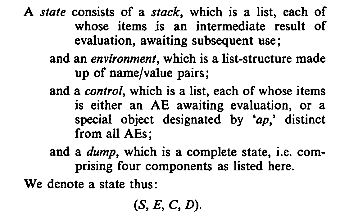
The most important piece of state is the control, which is a list of commands waiting to be executed, whereas the stack is a list of intermediate evaluation results. Each step of the machine updates parts of its state according to, mainly, the control, which says what to do next:
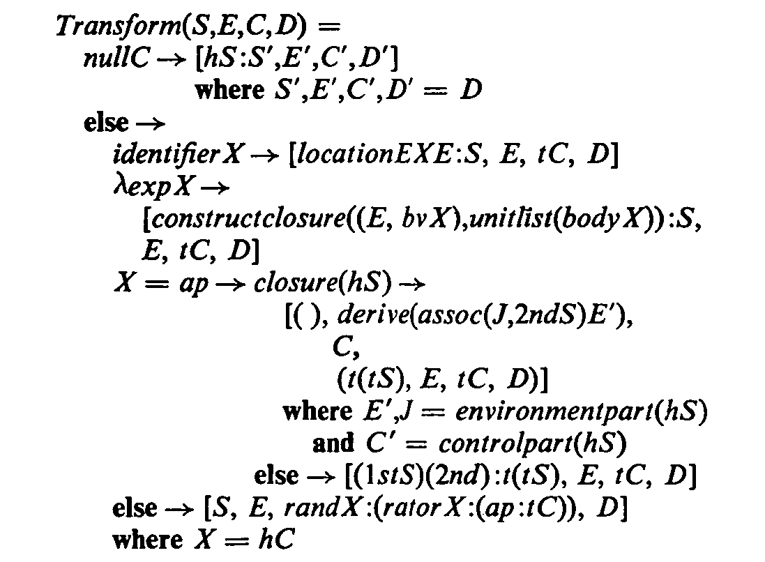
It was an incredibly influential contribution to show a toy machine that can evaluate expressions efficiently like this.
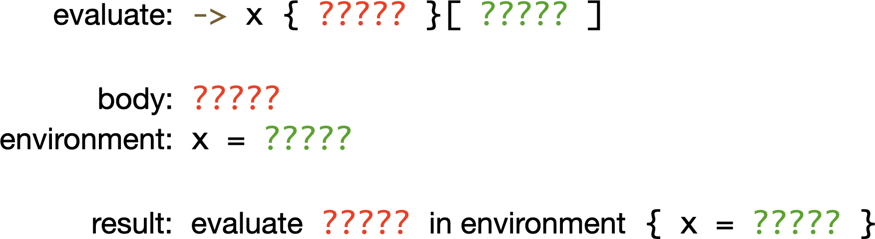
The mathematical description above is hard to read, so here’s a brief summary of how it works. What makes our implementation slow is all the reducing: we’re constantly rewriting the expression to replace variables with other larger expressions, and eventually the expressions get huge and it takes ages to do anything to them. Landin’s idea was instead to have the machine maintain something called an environment which remembers the names and values of all the variables currently in scope. Then we don’t need to do any rewriting: we can leave the expressions alone, and keep adding more names and values to the environment as we need to.
If we want to evaluate a proc definition being called with an argument, we pull out the body of that definition, and make a new environment which remembers that the parameter, x, should always have the value of whatever the argument was, and then we evaluate the body of the definition in that environment. We haven’t had to rewrite anything, we’ve just remembered the value of parameter x so that if we ever evaluate an occurrence of the variable x inside the body we can retrieve its value from the environment.
To make this environment idea work, the machine has to be careful about evaluating definitions, because the variable bindings in the current environment will probably be needed to evaluate the body of the definition later if it gets called. So Landin also invented a data structure called a closure that takes the definition and the current environment and wraps them together in a single value. That means I left out some detail in the previous paragraph: by the time a definition is called, it’s already been evaluated to a closure that has all of the variable bindings it needs to make sense of its body.
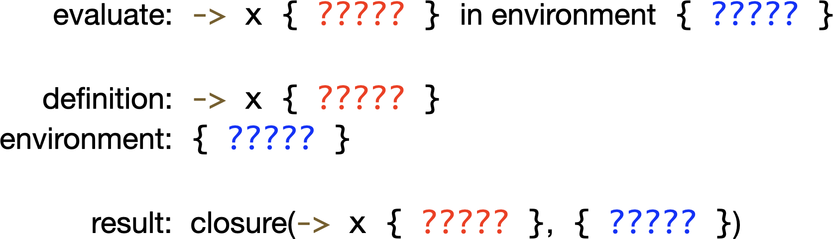
I won’t go into any more detail here but, essentially, environments and closures are why the SECD machine is faster than our expression rewriter.
Happily we can pretty much just write down the SECD machine’s transition function in Ruby:
Apply = Object.new
Closure = Struct.new(:environment, :definition)

def evaluate(expression)
  s, e, c, d = [], {}, [expression], nil

  loop do
    case { s: s, c: c, d: d }
    in c: [], d: nil, s: [result, *]
      return result
    in c: [], d: { s: s, e: e, c: c, d: d }, s: [result, *]
      s = [result] + s
    in c: [Variable(name), *c]
      s = [e.fetch(name)] + s
    in c: [Definition => definition, *c]
      s = [Closure.new(e, definition)] + s
    in c: [Closure | Constant => expression, *c]
      s = [expression] + s
    in c: [Apply, *c], s: [Closure(environment, Definition(parameter, body)), argument, *s]
      d = { s: s, e: e, c: c, d: d }
      s, e, c = [], environment.merge(parameter => argument), [body]
    in c: [Apply, *c], s: [receiver, argument, *s]
      s = [Call.new(receiver, argument)] + s
    in c: [Call(receiver, argument), *c]
      c = [argument, receiver, Apply] + c
    end
  end
end
This is a direct translation from the definition in the paper, with extra cases for evaluating closures and constants so that our technique for converting the results back to native integers works properly.
It’s definitely possible to write this more efficiently in Ruby by doing all the stack manipulation operations imperatively, calling the #push and #pop methods to destructively mutate the arrays, rather than using pattern matching to do it in a purely functional style…
Apply = Object.new
Closure = Struct.new(:environment, :definition)

def evaluate(expression)
  s, e, c, d = [], {}, [expression], nil

  loop do
    if c.empty?
      result = s.pop
      return result if d.nil?
      s, e, c, d = d.values_at(:s, :e, :c, :d)
      s.push(result)
    else
      case c.pop
      in Variable(name)
        s.push(e.fetch(name))
      in Definition => definition
        s.push(Closure.new(e, definition))
      in Closure | Constant => expression
        s.push(expression)
      in Apply
        case s.pop
        in Closure(environment, Definition(parameter, body))
          d = { s: s, e: e, c: c, d: d }
          s, e, c = [], environment.merge(parameter => s.pop), [body]
        in receiver
          s.push(Call.new(receiver, s.pop))
        end
      in Call(receiver, argument)
        c.push(Apply, receiver, argument)
      end
    end
  end
end
…but this is a bit messy and doesn’t correspond quite so nicely to the definition in the paper.
The SECD machine is quite a lot faster than what we were doing before: on my laptop it takes about three minutes rather than two hours to finish printing the FizzBuzz results. That’s around forty times faster.
That’s a good improvement, but can we make it even faster than that? Well, yes: because the SECD machine is a simple loop with a case statement inside it, it’s not too challenging to reimplement it in C. Then we can compile it down to native code instead of running it as interpreted Ruby, which should make it faster again.
In C we can declare a struct for representing an expression, which can be a variable, call, definition, closure or constant, and structs for representing the stack, environment, control and dump:
struct Expression {
  enum { Variable, Call, Definition, Closure, Constant } type;
  union {
    struct {
      char *name;
    } variable, constant;
    struct {
      struct Expression *receiver;
      struct Expression *argument;
    } call;
    struct {
      char *parameter;
      struct Expression *body;
    } definition;
    struct {
      struct Environment *environment;
      char *parameter;
      struct Expression *body;
    } closure;
  };
};

struct Stack {
  struct Expression *expression;
  struct Stack *rest;
};

struct Environment {
  char *name;
  struct Expression *expression;
  struct Environment *rest;
};

struct Control {
  enum { Expression, Apply } type;
  struct Expression *expression;
  struct Control *rest;
};

struct Dump {
  struct Stack *s;
  struct Environment *e;
  struct Control *c;
  struct Dump *d;
};
These are essentially four different flavours of linked list to keep things simple; in a more efficient implementation we’d allocate our own heap and store each structure contiguously as an actual stack so we can simply move a pointer up and down as it grows and shrinks.
We can translate the imperative version of the #evaluate method into C pretty directly. It’s got cases for how to handle the five kinds of expression, and the mechanism for updating the state when we apply a receiver to an argument:
struct Expression * evaluate (struct Expression *expression) {
  struct Stack *s = NULL;
  struct Environment *e = NULL;
  struct Control *c = push_control(NULL, Expression, expression);
  struct Dump *d = NULL;

  while (1) {
    if (c == NULL) {
      struct Expression *result = pop_stack(&s);
      if (d == NULL) return result;
      pop_dump(&s, &e, &c, &d);
      s = push_stack(s, result);
    } else {
      switch (c->type) {
        case Expression:
          {
            struct Expression *expression = pop_control(&c);

            switch (expression->type) {
              case Variable:
                s = push_stack(s, lookup(e, expression->variable.name));
                break;

              case Definition:
                s = push_stack(s, build_closure(e, expression->definition.parameter, expression->definition.body));
                break;

              case Closure:
              case Constant:
                s = push_stack(s, expression);
                break;

              case Call:
                c = push_control(c, Apply, NULL);
                c = push_control(c, Expression, expression->call.receiver);
                c = push_control(c, Expression, expression->call.argument);
                break;
            }
          }
          break;

        case Apply:
          {
            pop_control(&c);
            struct Expression *receiver = pop_stack(&s);
            struct Expression *argument = pop_stack(&s);

            switch (receiver->type) {
              case Closure:
                d = push_dump(s, e, c, d);
                s = NULL;
                e = push_environment(receiver->closure.environment, receiver->closure.parameter, argument);
                c = push_control(NULL, Expression, receiver->closure.body);
                break;

              default:
                s = push_stack(s, build_call(receiver, argument));
                break;
            }
          }
          break;
      }
    }
  }
}
To keep this code simple it doesn’t free any of the memory it allocates for environments or closures or new expressions, so in production code we’d need a garbage collector to clean up unused memory, but that’s a whole separate topic.
If we compile that C code into a dynamic library, we can use the ffi gem to connect it to Ruby. We just have to tell ffi what the C data structures look like and which C function to hook up as a Ruby method:
module SECD
  extend FFI::Library
  ffi_lib 'secd.so'

  enum :types, [:variable, :call, :definition, :closure, :constant]

  class Expression < FFI::Struct
    class Data < FFI::Union
      class Named < FFI::Struct
        layout name: :string
      end
      class Call < FFI::Struct
        layout receiver: Expression.ptr, argument: Expression.ptr
      end
      class Definition < FFI::Struct
        layout parameter: :string, body: Expression.ptr
      end
      class Closure < FFI::Struct
        layout environment: :pointer, parameter: :string, body: Expression.ptr
      end

      layout \
        variable: Named,
        call: Call,
        definition: Definition,
        closure: Closure,
        constant: Named
    end

    layout type: :types, data: Data
  end

  attach_function :evaluate, [Expression.by_ref], Expression.by_ref
end
We also have to write some helpers to convert Ruby abstract syntax trees to and from C structs so that we can pass them in and out of the #evaluate function, but that’s just boilerplate.
This C implementation of the SECD machine finishes executing FizzBuzz in one minute, so it’s three times faster than the Ruby version. That’s not a mindblowing improvement because the Ruby version was already relatively efficient, but still pretty good.
We were asking: could we make our implementation faster, and then even faster than that? And yes, we can, firstly by switching from an interpreter to a virtual machine, and then implementing the main loop of that machine in C instead of Ruby.
Here are what the timings look like:
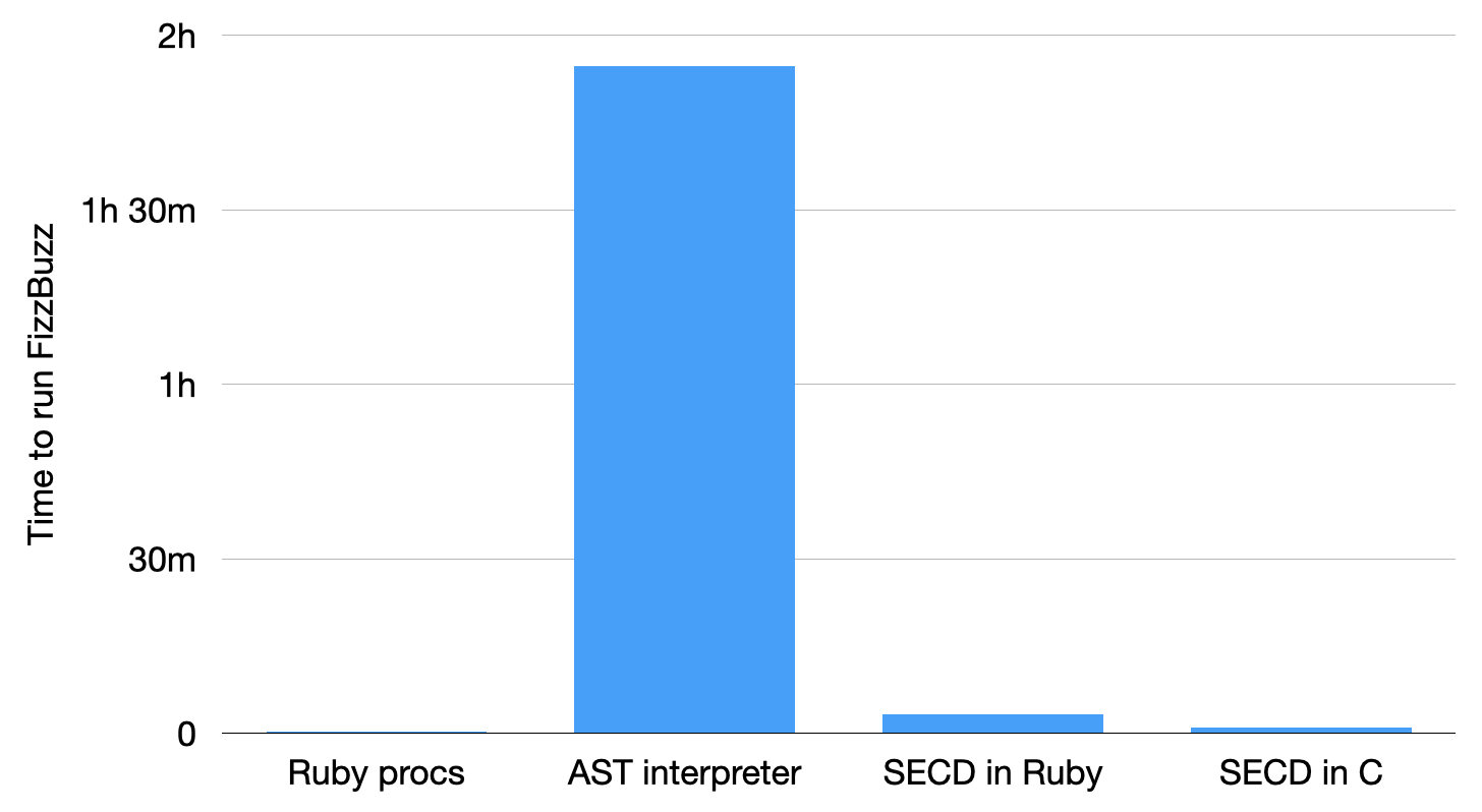
It’s a bit hard to see the detail because the interpreter is so much slower than everything else, so let’s zoom in a bit:
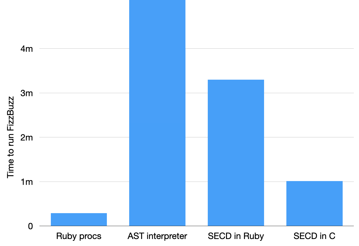
This shows that the SECD machine is starting to get close to the performance of Ruby procs, but it’s still about three times slower than what we started with.
This leads inductively to the obvious question: could we make this even faster still? Well, yes, there have been decades of subsequent work on how to make the original SECD machine faster.
For example, during execution the machine dynamically translates the original expression into a list of commands, but it’s easy to do that work ahead of time instead and compile the expression into commands in advance, which then allows the machine to run a lot faster and avoid the work of retranslating the bodies of expressions that get evaluated multiple times. The RubyVM::Compiled and NativeVM::Compiled implementations on GitHub demonstrate this idea, as well as showing how to eliminate the dump by incorporating it into the stack.
And to go further, once we have a list of commands for the machine to execute, we can translate each one directly into C or native machine code to avoid the need to interpret them at all. Given the NativeVM::Compiled implementation, it wouldn’t be much more work to convert the compiled instruction list into C source code and then use something like Inline to compile and run it.
What we’ve seen here are the first baby steps towards implementing a compiler for a simple functional language, and all those decades of research since the SECD machine was invented have uncovered many more tricks and optimisations we could use to make that compiler extremely efficient.
Ten years ago I concluded Programming with Nothing by asking: why? What’s the point of all this? On that occasion I said that we’d seen a tiny language which had the same computational power as Ruby despite being extremely minimal, and that the only fundamental difference between that minimal language and full Ruby is expressiveness, not power. What makes Ruby special to us is its particular flavour of expressiveness, and how it chooses to balance that against other concerns like performance, safety, simplicity and so on.
To answer the same question now: having previously seen how to write programs in a very restricted language, today we’ve seen how to actually implement that language for ourselves. This gives us the recipe for building and using our own programming language with the minimum features necessary to perform Turing-complete computation.
The previous talk showed that this language was sufficient to write any program; today we’ve seen that it can also be implemented in a couple of pages of code. From this realisation springs an entire history of implementations of functional languages, many of which are — more or less — an optimised and feature-enriched version of the basic SECD machine.
What we’ve seen here is just the beginning. A simple idea like the SECD machine is the starting point for a journey of iterative improvement that lets us eventually build a language that’s efficient, expressive and fast.
That’s everything I wanted to show you. The code is all available on GitHub if you want to read it, play with it and get a feel for how it works.
I hope you found some of that fun or interesting. I really appreciate your time and attention, so thanks very much for reading.